首页/文章/ 详情

DEFORM-2D操作指南

4月前浏览791

1.几何尺寸操作-XYR 格式

1.1创建新问题

1.2设置模拟控制

1.3创建新对象

1.4显示几何图形

1.5保存问题

1.6退出 DEFORM-2D 系统。

本章用到的图标。

image.png


1.创建新问题

1.1创建新问题

键入mkdir MESH 创建目录 Mesh,  并键入 cd MESH转向该目录。现在键入 DEFORM2 运行 DEFORM-2D,打 开DEFORM-2D 系统窗口(图1.1)。
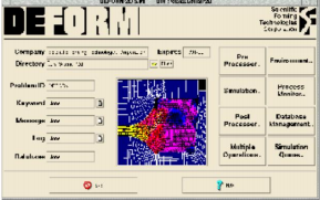
image.png

图1. 1-DEFORM-2D   System  窗口

在Problem   ID文本框中输入MESH, 完成以后进入 Pre-Processor      定义模拟数据。 单击 Pre-Processor      按钮打开包含有 Display    窗口,Contact    窗口和 Message  窗口的 Pre-Processor     窗口。
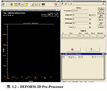
image.png

1.2设置模拟控制

单击 Control   窗口内的 Simulation     Control  按钮,打开模拟控制窗口,在 Simulation      Title  文本框中键入 Mesh 。设置单位为英制。选择 Geometry  为 Axisymmetric(轴对称),选择 Deformation (形变),关闭 Heat    Transfer(热传导),完 成后单击OK 按钮(图1.3)。
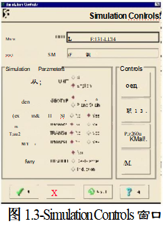
image.png

1.3创建新对象

选择 Control   窗口中的 Objects    按钮,打开 Objects    窗口,在本窗口中为所定的 对象设置数据,在这儿无需创建新对象。因为已有一缺省对象 object#1。
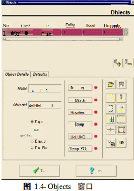

image.png

把 对 象 1 的 Object   name 设为 BILLET,Object   Type( 对象类型)为 Plastic    (塑性),现在单击 Geometry  按钮,来定义对象的几何尺寸(图1.5)。Geometry  窗口中包含有一 空白表,在一行空格输入数值后按 Enter  或 Tab 键可移向另一行,按住SHIFT键后按 TAB 可返回先前一行。现在单击 Apply  并输入 XYR 格式的下一来数值。

一旦你输完了所有数值,单击 Check   Geometry  按钮,若几何数据全部正确,会有 以下信息框出现。
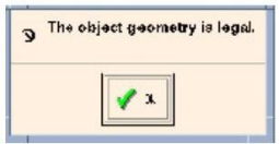
image.png

单击OK 按钮退出,并单击 Geometry  窗口中的 OK 按钮。Display     窗口会显示对象 的几何尺寸,即一圆柱 Billet。

1.4显示几何尺寸

用 Dynamic Zoom 和 Zoom Windows  按钮,可放大或缩小视图。

选择 Dynamic Zoom 按钮,激活动缩放功能。按住鼠标左键向上移会缩小,按住鼠 标左键向下移动会放大。同时,选用 Zoom Windows 按钮功能,可以缩放某一区域。单 击 Zoom Windows  按钮,在想放大区域的一角按下鼠标左键并拖定鼠标直至覆盖了该区 域,然后释放鼠标。另外用户可用 Pan  操作图形作全屏幕平移。单击 Dynamic Pan  按 钮。然后按住鼠标拖动视窗。

1.5保存问题

一旦完成对象数据输入后,应将当前数据保存到一个命令 Keyword 文件中。单击 Control  窗口中位于 Keyword 旁边的 Save   keyword   file图标,可数据存储。

另外,从 Control  窗口中的菜单 File→ Save  中,也可保存当前工作。

1.6退出 DEFORM-2D系统

单击 Control   窗口底部的 Exit  按钮,可退出该窗口。对于提示信息“Are  you  sure that    you    want    to    exit     the    pre-processor?” [ 你真想退了前处理吗?],单击 Yes 按 钮后再单击 DeFORM-2D 系统窗口中的 Exit  按钮退出。

2.几何尺寸输入X-IGES 文件

2.1创建新问题

2.2设置模拟控制

2.3创建新对象

2.3. 1对象1

2.3.2对象2

2.3.3对象3

2.4保存问题

2.5退出 DEFIORM-2D 系统。
image.png

2.几何尺寸输入X-IGES文件

2.1创建新问题

创建一 目录 SPIKE(mkdir    spike)并转向这一 目录,现在键入 DEFORM2  运行 DEFORM-2D 系统,并打开其窗口,在 Problem  ID 文本框中输入 SPIKE。完成后应进入 前处理部分定义模拟数据,单击Pre-Precessor     按钮,打开一包含 Display   窗口,Control    窗口和 Message    窗口的Pre-Processor      窗口。

2.2设置模拟控制

在单击 Control   窗口中的 Simulation-Control      按钮,打开其窗口,在 Simulation  Title    文本框中输入 SPIKE FORGING,设置单位为英制,选择 Deformation,  非选 Heat Transfer   项,选择 Geometry  为 Axisymmetric  完成后单击OK 按钮。

2.3创建新对象

2.3. 1对象1

单击 Control   窗口中的 Objects   按钮,打开 OBJECTS  窗口。窗口可定义选定对象 的数据,选中 Object  表中的缺省对象 object#1,     改变object#1    的名字(object  name)为 BILLET, 设置 OBJECT TYPE  为 PLASTIC  ( 塑性),现在单击 Geometry  按钮打开 Geometry 窗口。

本例输入的几何尺寸图形为 IGES  文件,因而单击 Geometry  窗口中的 Load IGES File  按钮,打开 IGES FILE SELECTION 窗口。(图2.1)

在文件列表中选中文件 BILLET.IGS, 并双击鼠标,单击 OK 按钮,打开 IGES 文件 输入窗口(图2.2)。

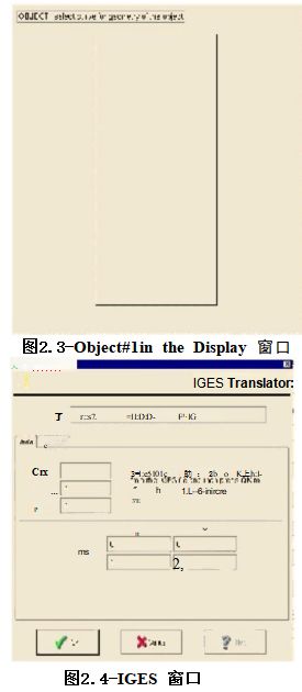
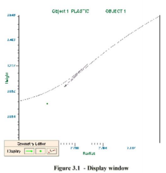
该窗口包含 IGES文件信息列表,由于缺省容差是合适的,因而单击OK按钮。Display  窗口中会有输入的 IGES格式几何图形(图2.3)的 IGES    Translator(IGES 转换器)窗口 (图2.4),对话框中列出了有关曲线、名称和点的数目。单击几何图形上的某一线可定 义你想输入的对象,对象的颜色由白色变为黄色。同样,也可定义曲线。
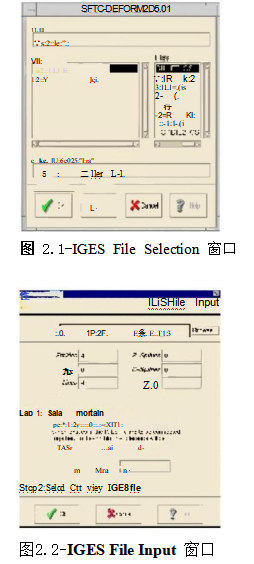
image.pngimage.png

单击 IGES TRANSLATOR 窗口中的OK 按钮,来输入所选择的曲线。Geometry  窗口中 的表列出了组成几何图形的一系列点。

Check Geometry  窗口中有 “ if  you   want   to   check   geometry” (你是否想检查几 何图形)的查询信息,单击Yes 按钮,如果一切正确,会有信息 “The  object  geometry is     legal”,的提示框出现,单击 OK 按钮,现在单击 Geometry 窗口中的OK按钮,Display   窗口会显示已输入的圆柱形 BILLET。

2.3.2对象2

单击 OBJECTS窗口中的 Add   Objects 按钮创建新对象 object#2 。 一标有 object#2的新对象会添加到 Object   表中,选中object#2   使之成红色,改变 object#2   名子为 TOP DIE后单击 Object   Geometry 按钮。

在有一空白表的 Geometry  窗口中单击右上角的Load  IGES  File 按钮,打开 IGES  File       Selection 窗口,在 Files    列表中选择 IGES 并双击该文件,现在单击 OK 按钮读 入该 IGES  文件。采用与 object#1     同样的步骤定义输入的曲线。一旦曲线输入完毕, 检查输入的几何尺寸并单击Yes 按钮,如果几何文件中的数据有错,并提示是否想更正, 单击Yes 按钮改正几何尺寸,最后单击 Geometry 窗口中的OK 按钮。

2.3.3对象3

单击 Add Object 按钮,创建新对象 object#3,    把 object#3    添加到 Object  表中, 选中表中的 object#3    使之成为红色,改变 object#3     的名字为 BOTTOM DIE  后,单击  Geometry 按钮,打开 Geometry 窗口。单击右上角的 Load  IGES  File  Input 按钮,输 入 IGES文件 BOTDIE.IGS,采用类似 object#1   和 object#2    的步骤定义要输入的曲线, 一旦曲线输入后检查几何尺寸,完成后单击 Object   窗口中的OK 按钮。

2.4保存问题:

一旦完成对象数据输入后,应将当前数据保存到一个命令 Keyword 文件中。单击 Control   窗口中位于 Keyword  旁边的 Save   keyword    file 图标,可数据存储。

另外,从 Control   窗口中的菜单 File→ Save   中,也可保存当前工作。

2.5退出 DEFORM-2D系统

单击 Control  窗口底部的 Exit  按钮,可退出该窗口。对于提示信息“Are you  sure that    you    want    to    exit    the    pre-processor?”[你真想退了前处理吗?],单击 Yes 按 钮后再单击 DeFORM-2D 系统窗口中的 Exit  按钮退出。

3.几何尺寸输入-几何修正

3.1打开-旧问题

3.2设置模拟控制

3.3创建新对象

3.4保存问题

本章使用图标

 image.png

3.几何输入-几何尺寸修正

3.1打开一先前保存的旧问题

创建目录 Junk ( 可通过命令 mkdir JUNK 实现)并转向这一目录,键入 DEFORM2运行 DEFORM-2D 系统,打开 DEFORM-2D窗口。在 Problem   ID文本框中输入 JUNK。完成后单 击 Pre-Proccessor按钮,开始前处理过程。

3.2设置模拟控制

单击 Control   窗口中的 Simulation      Control 按钮打开 Simulation       Control 窗口, 在 Simulation       Title 文本框中输入 JUNK。设置单位为英制,选择 Deformation,    关闭 Heat  Transfer,      设置 Geometry  为 Axisymmetric 。 完成后单击OK 按钮。

3.3. 创建一新问题

单击 Control    窗口中的 Objects    按钮,打开 Object    窗口,改变 object#1     为 BILLET。设置 TYPE 为 Plastic 。 现在单击 Geometry 按钮打开一有空白表格的 Geometry 窗口,输入下表中的 XYR 坐标值。
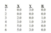
image.png

image.png

注意连接处的两段圆弧,用 Zoom窗口按钮放大这一区域,由于IGES文件格式中的 数据缺陷,曲线没有完全接触,出现了折叠。单击 Geometry 窗口中的 Check  Geometry 按钮,会有以下信息框。
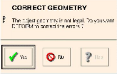
image.png

单击Yes 按钮,修正几何尺寸, DEFORM-2D会自动改变圆弧半径直至端点平滑过渡, 完成后单击 OK按钮。最后单击 Object   窗口中的OK 按钮。

3.4保存问题

一旦完成对象输入后应保存数据到 Keyword  文件。单击 Control    窗口中位于 Keyword 旁边的 Save   keyword    file图标,完成数据存储任务。

另外,从 Control   窗口中的菜单 File→ Save,     也可保存当前工作。

3.5退出 DEFORM-2D系统

单击 Control   窗口底部的 Exit  按钮,可退出该窗口。对于提示信息“Are  you  sure that    you    want    to    exit     the    pre-processor?” [ 你真想退了前处理吗?],单击 Yes 按 钮后再单击 DeFORM-2D系统窗口中的 Exit  按钮退出。

详细内容请见附件


免责声明:


本页面/内容部分素材来源于互联网公 开 信 息,旨在传递更多信息,不代表本平台立场。

版权归原作者或机构所有,如涉及侵权,请通过平台联系我们,我们将在核实后第一时间处理。

本平台对转载内容的真实性、准确性不作任何保证,用户需自行判断并承担使用风险。

附件

免费P7-DEFORM-2D操作指南.pdf
ACTSystemDeform控制
著作权归作者所有,欢迎分享,未经许可,不得转载
首次发布时间:2026-06-02
最近编辑:4月前
仿真支持爱好者
在仿真的路上越走越远
获赞 333粉丝 26文章 318课程 0
点赞
收藏
作者推荐

高温 H₂-CO 氧化动力学模型优化分析(h2-co)

摘要:本文构建并优化了高温 H₂-CO 燃烧详细动力学模型,整合最新热力学、反应速率与输运参数,包含 14 种组分、30 步基元反应。以激波管点火延迟、层流火焰速度、流动反应器组分浓度及火焰结构等 36 组实验为优化目标,对 28 个关键反应指前因子与三体效率进行系统优化。重点修正 H+O₂+M、CO+OH 等核心反应速率,显著提升模型预测精度。优化模型可准确复现宽工况(880–2625 K、0.3–33 atm)下的燃烧特性,为氢 - 一氧化碳混合燃料的数值模拟提供可靠动力学基础。An optimized kinetic model of H2/CO combustionScott G. Davisa,*, Ameya V. Joshia, Hai Wanga, Fokion Egolfopoulos ba Department of Mechanical Engineering, University of Delaware, Newark, DE 19716, USAb Department of Aerospace and Mechanical Engineering, University of Southern California, Los Angeles, CA 90089, USAAbstractWe propose a H2–CO kinetic model which incorporates the recent thermodynamic, kinetic, and species transport updates relevant to high-temperature H2 and CO oxidation. Attention has been placed on obtaining a comprehensive and kinetically accurate model able to predict a wide variety of H2–CO com- bustion data. The model was subject to systematic optimization and validation tests against reliable H2– CO combustion data, from global combustion properties (shock-tube ignition delays, laminar flame speeds, and extinction strain rates) to detailed species profiles during H2 and CO oxidation in flow reactor and in laminar premixed flames.◎ 2004 The Combustion Institute. Published by Elsevier Inc. All rights reserved.Keywords: Kinetics; Detailed reaction model; Hydrogen; Carbon monoxide1. IntroductionThe most successful model of H2–CO combus- tion has been that of Mueller et al. [1], developed on the basis of a careful evaluation of relevant ki- netic parameters and flow reactor experiments. The model is also able to predict a wide range of flame experiments. Over the last few years, however, the rate parameters of the key reaction H + O2 + M = HO2 + M and its third-body effi- ciencies have been revised [2,3], giving an urgent reason for a re-examination of the H2–CO com- bustion model. The downward revision of the en- thalpy of formation of OH [4] may also exert an influence on the overall reaction kinetics of H2 combustion.Several new studies [5–7] have been reported in recent years. Two of these studies a nalyzed the hydrogen submodel [5,6], both being an extension of the model of Mueller et al. The third an alysis [7] considered both H2 and CO chemistry and is the predecessor to the present study. The objec- tives of the present study are (1) to provide an up- date for the H2–CO combustion reaction model on the basis of recent kinetic data, and (2) to opti- mize the H2–CO model against available H2–CO combustion data.2. Reaction modelThe unoptimized (trial) reaction model consists of 14 species and 30 reactions as shown in Fig. 1. The model and its thermochemistry and transport property files can be found at the URL: http:// ignis.me.udel.edu/h2co. The trial model was based on a careful review of recent kinetics literature, considering both direct data and compilations. A large number of GRI 3.0 rate parameters [8] were found to be appropriate and are used. The discus- sion below highlights the choice of key rate parameters.Fig. 1. Trial reaction model of H2–CO oxidation, active parameters, and their spans employed in model optimization (see Refs. [9,14,16–18]).The rate expression of H + O2 = O + OH was taken from GRI 3.0 [8]. The rate coeffi- cient of H + O2(+M) = HO2(+M) was based on Troe [2], who employed a high-pressure rate krec,∞ (cm3 mol__1 s__1) = 4.65 × 10¹² T0.44 and developed the low-pressure and fall-off expres- sions for Ar and N2 as the bath gases. The broad- ening factor Fc was found to be 0.5 for both third bodies. Troe’s fall-off rate parameterization, how- ever, could not be directly used in CHEMKIN [19], because the low-pressure limit rate coefficient k0 does not share the same temperature depen- dence for different third bodies. We had to devel- op parameterized rate expressions (see Fig. 1) based on the k0 expression of Ar and using the fall-off formula of Troe [20]. A collision efficiency factor β = 0.53 was used for Ar relative to N2. The collision efficiency of He was assumed to be equal to that of Ar. The study of Michael et al.[3] supports a collision efficiency of O2 s maller than that of N2. We found that for O2, β = 0.75 gives a good agreement with experiment [3] and theory [2]. For H2O, Troe [2] suggested that the broadening factor is close to the strong-collision limit. We chose a β value of 12 (relative to N2) with the resulting rate in good agreement with those of Troe and others [2,3,21].The k0 expression of H + OH + M = H2O + M was taken from [8] with the β values equal to 0.38 and 6.3 for Ar and H2O, respectively [12]. The rate expression of Michael et al. [10] was employed for H2 + O2 = H + HO2. For OH + OH(+M) = H2O2(+M), the k0 expression, given in the reverse direction by Baulch et al.[12], was refitted based on the new heat of forma- tion of the OH radical along with the low temper- ature data of Zellner et al. [11]. The krec,∞ expression and the β value of H2O (6) were taken from [11] while the Troe fall-off parameters [22] were the same as those in GRI 3.0. The rate expressions for H2O2 + OH = HO2 + H2O were taken directly from [15], though the high-temper- ature expression was refitted using a modified Arrhenius expression to avoid the rate constant values exceeding the collision limit when extrapo- lated to high temperatures.For CO + O(+M) = CO2(+M), the k∞ expres- sion was taken from [13], and following Allen et al. [23], k0 was taken from the QRRK ana lysis of Westmoreland et al. [24] and fall-off was that of Lindemann. The collision efficiency of H2O was assumed to be 12. The rate constant for CO + OH = CO2 + H was re-an alyzed in the present study, and the experimental data were refitted by the sum of two modified Arrhenius expressions. The new expression resolves more accurately the high temperature data of Woold- ridge et al. [25] as well as the data found in [26]. Without this revision, it was not possible to recon- cile the high-temperature H2 ignition data with the H2–CO laminar flame speeds. The known pressure dependence of this reaction was not con- sidered as this dependence is quite unimportant for the CO oxidation experiments considered herein. 3. Computational and optimization methodA comprehensive review was conducted for a large number of H2–CO combustion data. Thir- ty-six experiments were chosen as optimization targets as shown in Table 1. They can be classified into four categories: (1) laminar flame speeds of H2–air, H2–O2–He, and H2–CO–air mixtures, (2) the peak mole fractions of H and O in a low-pres- sure burner-stabilized H2–O2–Ar flame, (3) the consumption rates of H2 and CO during the reac- tion of H2–O2–N2 and CO–O2–H2O–N2 mixtures in a turbulent flow reactor, and (4) ignition delay times of H2–O2–Ar and H2–CO–O2–Ar mixtures behind reflected shock waves.Ignition delay and flow reactor calculations were conducted using a kinetic integrator inter- faced with CHEMKIN [19] by assuming adiabatic condition. Ignition delays were modeled using the constant-density model, whereas flow reactor modeling used the constant-pressure assumption. The numerical ignition delays were determined following the same ignition criteria as in the respective experiments. Laminar flame speeds and structure were calculated using Premix [40], employing thermal diffusion, and multicomponent transport. Diffusion coefficients of several key pairs were updated [41].Sensitivity an alyses were conducted for igni- tion delay and consumption rates of the fuel in flow reactor with a brute force method. For lam- inar flame speeds and H and O peak mole frac- tions in burner-stabilized flames, the local sensitivity methods were utilized. Based on the sensitivity information, active rate parameters (to be optimized) were chosen for each target. The entire set of active parameters consists of 28 A-factors and third-body efficiency factors as shown in Figs. 1 and 2.The optimization approach is similar to earlier studies [8,43]. Briefly, the solution mapping tech- nique was employed to express a response by a sec--ijp, a’sl n(2d) ’0a1iii1,x’s are factorial active variables given by x = ln (a/atrial)/ln (f), where a is the active A factor or third-body efficiency factor, and f is its span or uncertainty factor. The uncertainty factor was esti- mated on the basis of kinetic uncertainty and is pro- vided in Fig. 1 for each active parameter. Though an optimization of the temperature dependence of rate coefficients is possible, we chose not to vary the T-dependence because of the insufficient num- ber of systematic experimental targets [43].For flow reactor targets, the response was found to be highly non-linear with respect to x’s. These responses are expressed by adding a hyper- bolic tangent term to account for the S-shaped dependence of response with respect to x’s,η = η(2) + ctanh(a +Σ= 1 axi +Σ1 Σ≥ibxixj). The coefficients for the flow reactor and igni- tion delay targets were calculated by a factorial design test [43]. The coefficients for flame targets were obtained using the sensitivity an alysis based method [44].Minimization was carried out on the objective function L2 = Σi[(ηi,expt __ ηi,calc)/σi]2 subject to the constraint __1 < {x} < +1, where the subscript i denotes the ith target. Each target was individually weighted by their uncertainty σi . The target values and their uncertainties are presented in Table 1.4. Results and discussionThe trial kinetic model was tested against a wide range of experimental data. The predictions of the trial model for the 36 target values are shown in Table 1 (the ‘‘trial’’ column). Overall the model performed well against these experi- mental data. The exceptions are: it overpredicts H2–O2–He flame speeds, the H and O mole frac- tions in the burner-stabilized flame, and the consumption rate of H2 for the 1.0% H2–1.5 O2%–N2 flow reactor mixture at 943 K and 2.5 atm.To reconcile these discrepancies, optimization was then carried out for 28 active parameters with respect to 36 targets. All active parameters were allowed to vary freely within their uncertainty spans. The optimal parameter set was obtained as the minimum of L2, first from a random sample of the multidimensional parameter space, fol- lowed by a Newton search of the L2 minimum in the parameter space. The values of optimized active parameters are shown in the last column of Fig. 2 (expressed as the optimized-to-trial parameter ratio). To obtain the optimized model, the active parameters (A-factors and third-body efficiency factors) shown in Fig. 1 should be mul- tiplied by their corresponding ratios.Validation of the optimized model will be dis- cussed below. Figure 3 presents experimental [27–31,45] and computed laminar flame speeds of H2–air and air-equivalent mixtures where N2 was replaced by Ar or He. With trial model predictions already close to the experimental values, the opti- mization served only to fine-tune the model, result- ing in excellent agreement with the experiment as can be seen in Fig. 3 and Table 1. The trial model tends to overpredict the H2–O2–He flame speeds at elevated pressures (Table 1). The discrepancies are clearly caused by kinetics as a previous study showed that the uncertainty in the transport coeffi- cients cannot account for the observed differences [41]. Now the optimized model can successfully pre- dict these H2–O2–He flame speeds [27] as seen in Fig. 4. This agreement was brought by lowering the rate of OH + H2 = H + H2O, H + HO2 = OH + OH, and a s mall increase in the rate of H + O2 + H2O = HO2 + H2O.The dominant sensitivity of the laminar flame speeds of H2–CO–air mixtures, especially the 95% CO + 5% H2 mixtures, to CO + OH = CO2 + H has been observed elsewhere [32] and necessitated a re-evaluation this reaction. It was determined that the sum of two modified Arrhe- nius expressions was necessary to predict the lam-the optimized model reproduces experimental H2–CO–air laminar flame speeds [32,33].Figure 7 depicts species profiles for four se- lected H2 oxidation experiments in a turbulent flow reactor [13]. Time shift was necessary to match the computed profiles with the experimen- tal counterparts. The amounts of time shift were found to be similar with those used by Mueller et al. [13]. It is seen that the optimized model pre- dicts the experimental species profile accurately, and it also improved the prediction of the experi- ment as compared to the trial model (cf. Fig. 7B). Similarly, the results of Fig. 8 show that for CO oxidation [35] the optimized model accurately pre- dicts the CO consumption rate over an extended pressure range.Fig. 2. Target-active parameter matrix.Fig. 3. Experimental (symbols) and computed (lines: the optimized model) H2–air and air equivalent (N2 is replaced by Ar or He) flame speed at a pressure of 1 atm.Fig. 4. Experimental (symbols [27]) and computed (lines: the optimized model) H2–O2–He flame speeds.The trial model could accurately reconcile most of the ignition delay data for H2–O2–diluent mixtures, and optimization served only to im- prove these predictions as can be seen in Table 1. In addition, Fig. 9 shows a plot of experimental and computed ignition delay times for H2–O2–Ar mixtures [36–38,46] behind reflected shock waves. Here, the experimental shock-tube ignition delay data were fitted into τ (μs) = [H2]__0.154[O2]__0.693 [Ar]0.04 [6.77 × 10__8 T0.252 e9234/T] for non-‘‘run-Fig. 5. Experimental (symbols [32]) and computed (lines: the optimized model) H2–CO–air flame speeds at a pressure of 1 atm.Fig. 6. Experimental (symbols [33]) and computed (lines: the optimized model) H2–CO–air flame speeds at a pressure of 1 atm.Fig. 7. Experimental (symbols [13]) and computed (lines) species mole fraction profiles during hydrogen oxidation in a flow reactor. Solid lines: optimized model; dashed lines: trial model.Fig. 8. Experimental (symbols [35]) and computed (lines) [CO]/[CO]0 profiles during moist CO oxidation in a flow reactor. Cases (a): 1.014% CO + 0.517% O2 + 0.65% H2O in N2, p = 1 atm, T0 = 1038 K, (b) 1.01% CO + 0.496% O2 + 0.65% H2O in N2, p = 2.44 atm, T0 = 1038 K, (c) 0.988% CO + 0.494% O2 + 0.65% H2O in N2, p = 3.46 atm, T0 = 1038 K, (d) 0.984% CO + 0.497% O2 + 0.65% H2O in N2, p = 6.5 atm, T0 = 1040 K, and (e) 0.994% CO + 1.47% O2 + 0.65% H2O in N2, p = 9.6 atm, T0 = 1039 K.Fig. 9. Experimental (symbols) and computed (lines) ignition delay times of H2–O2–Ar mixtures behind reflected shock waves. Symbols: (a) 6.67% H2 + 3.33% O2, p5 = 1.35–2.90 atm; (b) 5% H2 + 5% O2, p5 = 1.35– 2.90 atm (onset of pressure rise [36]), (c) 0.5% H2 + 0.25% O2, p5 = 33 atm, (d) 2% H2 + 1% O2, p5 = 33 atm, (e) 0.5% H2 + 0.25% O2, p5 = 57 atm, (f) 0.33% H2 + 0.17% O2, p5 = 64 atm, (g) 0.1% H2 + 0.05% O2, p5 = 64 atm, (h) 0.5% H2 + 0.25% O2, p5 = 87 atm (maximum OH absorption rate [38]), (i) 8% H2 + 2% O2, p5 = 5 atm (maximum OH emission) [46], and (j) four H2 + O2 mixtures [37]. Lines: (1) 0.5% H2 + 0.25% O2, p5 = 87 atm (maximum [OH] rate), (2) 2% H2 + 1% O2, p5 = 33 atm (maximum [OH] rate), (3) 8% H2 + 2% O2, p5 = 5 atm (maximum [OH]), and (4) 5% H2 + 5% O2, p5 = 2 atm (maximum pressure gradient).Fig. 10. Experimental (symbols) and computed (lines) ignition delay times behind reflected shock waves for H2–O2–N2 mixtures. Experimental data were determined from onset of pressure rise [47] and maximum rate of OH emission [48].详细内容请见附件免责声明:本页面/内容部分素材来源于互联网公 开 信 息,旨在传递更多信息,不代表本平台立场。版权归原作者或机构所有,如涉及侵权,请通过平台联系我们,我们将在核实后第一时间处理。本平台对转载内容的真实性、准确性不作任何保证,用户需自行判断并承担使用风险。

有附件
未登录
还没有评论
课程
培训
服务
行家
VIP会员 学习计划 福利任务
下载APP
联系我们
帮助与反馈