计算流体动力学:原理与应用(第三版)核心内容梳理

计算流体动力学:原理与应用(第三版)核心内容梳理(Computational Fluid Dynamics Principles and Applications, Third Edition 3rd Edition)
摘要:
本文是 Jiri Blazek 所著 CFD 经典教材第三章、第四章核心内容,系统阐述 CFD 控制方程数值求解框架,梳理有限差分、有限体积、有限元等主流空间离散方法,对比结构化与非结构化网格适配特性。重点详解有限体积法,划分单元中心、顶点重叠、对偶控制体积三类格式,剖析中心、矢通量分裂、Roe 格式等对流离散方案,介绍显式 / 隐式时间推进、多重网格加速、各类湍流模型与边界条件处理思路。完整给出二维、三维结构化网格几何量计算方法,推导多种通量离散公式,兼顾理论推导与工程实现,系统讲解高精度插值、限制器、预处理等关键数值技术,是可压缩流动仿真算法的权威理论参考。
ACKNOWLEDGMENTS
My first thanks are to our Creator, without whom nothing would be possible. Furthermore, I wish to thank my father for the initial motivation to start this project, as well as for his continuous help with the text and in particular with the drawings. I also gratefully acknowledge the support of the staff at Elsevier Ltd., foremost of C. Owen and H. Gray, during the preparation of this edition.
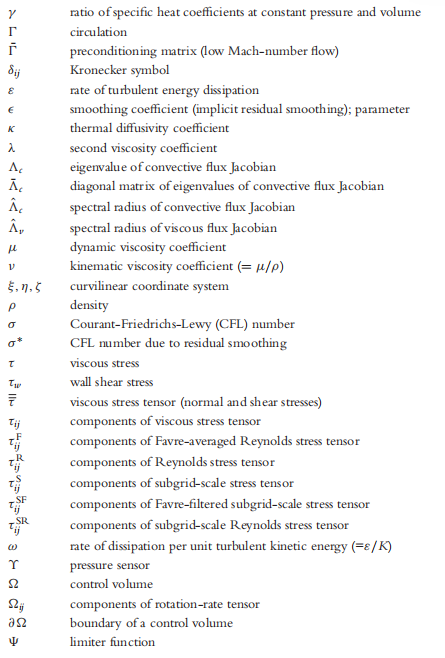
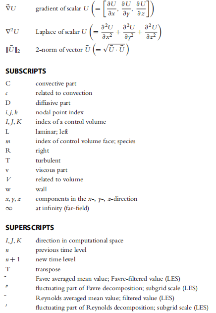
LIST OF SYMBOLS
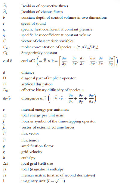
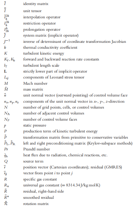
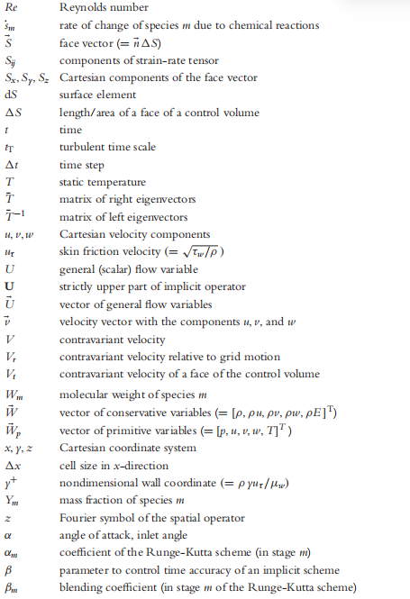
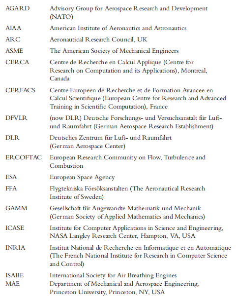
ABBREVIATIONS
CHAPTER 1 Introduction
The history of the computational fluid dynamics (CFD) started in the early 1970s. Around that time, it became an acronym for the combination of physics, numerical mathematics, and, to some extent, computer sciences—all employed to simulate fluid flows. The beginning of CFD was triggered by the availability of increasingly more powerful mainframes, and still the advances in CFD are closely linked to the evolution of the computer technology. Among the first applications of the CFD methods was the simulation of transonic flows based on the solution of the non-linear potential equation. With the beginning of the 1980s, first the solutions of two-dimensional (2-D) and later three-dimensional (3-D) Euler equations became feasible. Thanks to the rapidly increasing speed of supercomputers, and due to the development of a variety of numerical acceleration techniques like multigrid, it became possible to compute inviscid flows either past complete aircraft configurations or inside of turbomachinery. With the mid-1980s, the focus started to shift to the significantly more demanding simulations of viscous flows governed by the Navier-Stokes equations. Together with this, a variety of turbulence models evolved with different degree of numerical complexity and accuracy. The leading edge in turbulence modeling is represented by the direct numerical simulation and the large eddy simulation (LES).
With the advances of the numerical methodologies, particularly of the implicit schemes, solution offlow problems that require real gas modeling also became feasible by the end of the 1980s. Among the first large scale application, 3-D hypersonic flow past re-entry vehicles, like the European HERMES shuttle, was computed using equilibrium and later non-equilibrium chemistry models. Many research activities were and still are devoted to the numerical simulation of combustion and particularly to flame modeling. These efforts are very important for the development of low emission gas turbines and engines. Also, the modeling of steam and in particular condensation of steam became a key factor in designing efficient steam turbines.
Due to the steadily increasing demands on the complexity and the fidelity of flow simulations, grid generation methods became more and more sophisticated. The development started first with relatively simple structured meshes, constructed either by algebraic methods or by using partial differential equations. But with the increasing geometrical complexity of the configurations, the grids had to be divided into a number of topologically simpler blocks (multiblock approach). The next logical step was to allow for non-matching interfaces between the grid blocks, in order to relieve the constraints
imposed on the grid generation in a single block. Finally, solution methodologies were introduced that can deal with grids overlapping each other (Chimera technique). This allowed, for example, to simulate the flow past the complete Space Shuttle vehicle with the external tank and boosters attached. However, the generation of a structured, multiblock grid for a complicated geometry may still take weeks to accomplish. Therefore, the research also focused on the development of unstructured grid generators and flow solvers, which promise significantly reduced setup times, with only a minor user intervention. Another very important feature of the unstructured methodology is the possibility of solution-based grid adaptation. The first unstructured grids consisted exclusively of isotropic tetrahedra, which was fully sufficient for inviscid flows governed by the Euler equations. However, the solution of the Navier-Stokes equations at higher Reynolds numbers requires grids, which are highly stretched in the shear layers. Although such grids can also be constructed from tetrahedral elements, it is advisable to use pris ms or hexahedra in the viscous flow regions and tetrahedra outside. This improves not only the solution accuracy, but it also saves the number of elements, faces, and edges. Thus, the memory and run-time requirements of the simulation are reduced significantly.
Nowadays, CFD methodologies are routinely employed in the fields of aircraft, turbomachinery, car, and ship design. Furthermore, CFD is also applied in meteorology, oceanography, astrophysics, biology, oil recovery, and in architecture. Many numerical techniques developed for CFD are also utilized in the solution of the Maxwell equations or in aeroacoustics. Hence, CFD has become an important design tool in engineering, and also an indispensable research tool in various sciences. Due to the advances in numerical solution methods and in the computer technology, geometrically and physically complex cases can be run even on PCs or on PC clusters. Large scale simulations of viscous flows on grids consisting of dozens of millions of elements can be accomplished within only a few hours on today’s supercomputers. However, it would be completely wrong to think that CFD represents a mature technology now, like, for example, the finite-element methods in solid mechanics. No, there are still many open questions like turbulence and combustion modeling, heat transfer, efficient solution techniques for viscous flows, robust but accurate discretization methods, automated grid generators, etc. The coupling between CFD and other disciplines (like the solid mechanics) requires further research as well. Quite new opportunities also arise in the design optimization by using CFD.
The objective of this book is to provide university students with a solid foundation for understanding the numerical methods employed in today’s CFD and to familiarize them with modern CFD codes by hands-on experience. The book is also intended for engineers and scientists starting to work in the field of CFD, or who are applying CFD codes. The mathematics used is always connected to the underlying physics to
facilitate the understanding of the matter. The text can serve as a reference handbook too. Each chapter contains an extensive bibliography, which may form the basis for further studies.
CFD methods are concerned with the solution of equations of fluid motion as well as with the interaction of the fluid with solid bodies. The equations governing the motion of an inviscid fluid (Euler equations) and of viscous fluid (Navier-Stokes equations) are derived in Chapter 2. Additional thermodynamic relations for a perfect gas as well as for a real gas are also discussed. Chapter 3 deals with the principles of solution of the governing equations. The most important methodologies are briefly described and the corresponding references are provided. Chapter 3 can be used together with Chapter 2 to get acquainted with the fundamental principles of CFD.
Numerous schemes were developed in the past for the spatial discretization of the Euler and the Navier-Stokes equations. A unique feature of the present book is that it deals with both the structured (Chapter 4) as well as with the unstructured finite-volume schemes (Chapter 5), because of their broad application possibilities, especially for the treatment of complex flow problems routinely encountered in an industrial environment. The attention is particularly devoted to the definition of the various types of control volumes together with spatial discretization methodologies for convective and viscous fluxes. The 3-D finite-volume formulations of the most popular central and upwind schemes are presented in detail.
The methodologies for the temporal discretization of the governing equations can be divided into two main classes. One class comprises explicit time-stepping schemes (Section 6.1), and the other one consists of implicit schemes (Section 6.2). In order to provide a more complete overview, recently developed solution methods based on the Newton-iteration as well as standard techniques like the explicit Runge-Kutta schemes are discussed.
Two qualitatively different types of viscous fluid flows are encountered in general: laminar and turbulent. The solution of the Navier-Stokes equations does not raise any fundamental difficulties in the case of laminar flows. However, the simulation of turbulent flows continues to present a significant challenge as before. A relatively simple way of modeling the turbulence is offered by the so-called Reynolds-averaged Navier-Stokes equations. On the other hand, Reynolds stress models or LES enable considerably more accurate predictions of turbulent flows. In Chapter 7, various well-proven and widely applied turbulence models of varying level of complexity are presented in detail.
In order to account for the specific features of a particular problem, and to obtain an unique solution of the governing equations, it is necessary to specify appropriate boundary conditions. Basically, there are two types of boundary conditions: physical and numerical. Chapter 8 deals with both types in different situations like solid walls, inlet, outlet, injection, and far-field. Symmetry planes, periodic and block boundaries are treated as well.
In order to reduce the computer time required to solve the governing equations for complex flow problems, it is quite essential to employ numerical acceleration techniques. Chapter 9 deals extensively, among others, with approaches like the implicit residual s moothing and multigrid. Another important methodology which is also described in Chapter 9 is preconditioning of the governing equations. It allows the application of a single numerical scheme for flows, where the Mach number varies between nearly zero and transonic or higher values. Finally, Chapter 9 contains a section on the parallelization of numerical computer codes by using different approaches.
Each discretization of the governing equations introduces a certain error—the discretization error. Several consistency requirements have to be fulfilled by the dis- cretization scheme, in order to ensure the solution of the discretized equations closely approximates the solution of the original equations. This problem is addressed in the first two parts of Chapter 10. Before a particular numerical solution method is implemented, it is important to know, at least approximately, how the method will influence the stability and the convergence behavior of the CFD code. It was frequently confirmed that the Von Neumann stability an alysis can provide a good assess ment of the properties of a numerical scheme. Therefore, the third part of Chapter 10 deals with stability an alysis for various model equations.
One of the challenging tasks in CFD is the generation of structured or unstructured body-fitted grids around complex geometries. The grid is used to discretize the governing equations in space. The accuracy of the flow solution is therefore closely linked to the quality of the grid. In Chapter 11, the most important methodologies for the generation of structured as well as unstructured grids are discussed in depth.
In order to demonstrate the practical aspects of different numerical solution method- ologies, various source codes are available for download. Provided are the sources of quasi 1-D Euler, as well as of 2-D Euler and Navier-Stokes structured and unstructured flow solvers. Furthermore, source codes of 2-D structured algebraic and elliptic grid generators are included together with a converter from structured to unstructured grids. Furthermore, two programs are provided to conduct the linear stability an alysis of explicit and implicit time-stepping schemes. The source codes are completed by a set of worked out examples including the grids, the input files and the results. The code package also contains several programs for the demonstration of parallelization techniques. Chapter 12 describes the contents ofthe directories, the capabilities of the particular programs, and provides examples of their usage.
The present book is finalized with an Appendix and Index. The Appendix contains the governing equations presented in a differential form as well as their characteristic properties. Formulations of the governing equations in rotating frame of reference and for moving grids are discussed along with some simplified forms. Furthermore, Jacobian and transformation matrices from conservative to characteristic variables are presented for two and three dimensions. The GMRES conjugate gradient method for the solution of linear equations systems is described next. The Appendix closes with a brief explanation of the tensor notation.
原资料见附件
免责声明:
本页面/内容部分素材来源于互联网公 开 信 息,旨在传递更多信息,不代表本平台立场。
版权归原作者或机构所有,如涉及侵权,请通过平台联系我们,我们将在核实后第一时间处理。
本平台对转载内容的真实性、准确性不作任何保证,用户需自行判断并承担使用风险。