基于详细化学机理的柴油喷雾燃烧与 NOx 及碳烟模拟(zheng DME_mech)

摘要:
本文基于详细化学反应与现象学碳烟模型,构建柴油喷雾火焰 CFD 仿真模型,采用正庚烷骨架机理耦合简化 NOₓ机理,结合 KIVA-3V 与 CHEMKIN 求解燃烧与排放。模型以乙炔为碳烟前驱体,模拟碳烟生成与氧化过程,经 Sandia 燃烧室与卡特彼勒柴油机实验验证。结果准确预测火焰浮起长度、碳烟分布及排放趋势,证实减小喷孔直径、降低环境温度可抑制碳烟;推迟喷油能同步降低 NOₓ与碳烟。该模型可用于 PCCI 低温燃烧分析,为低排放柴油机设计提供数值工具。
Modeling Diesel Spray Flame Liftoff, Sooting Tendency,and NOx Emissions Using Detailed Chemistry WithPhenomenological Soot Model
A detailed chemistry-based CFD model was developed to simulate the diesel spray com- bustion and emission process. A reaction mechanis m of n-heptane is coupled with a reduced NOx mechanis m to simulate diesel fuel oxidation and NOx formation. The soot emission process is simulated by a phenomenological soot model that uses a competing formation and oxidation rate formulation. The model is applied to predict the diesel spray lift-off length and its sooting tendency under high temperature and pressure con- ditions with good agreement with experiments of Sandia. Various nozzle diameters and chamber conditions were investigated. The model successfully predicts that the sooting tendency is reduced as the nozzle diameter is reduced and/or the initial chamber gas temperature is decreased, as observed by the experiments. The model is also applied to simulate diesel engine combustion under premixed charge compression ignition (PCCI) conditions. Trends of heat release rate, NOx, and soot emissions with respect to EGR levels and start-of-injection timings are also well predicted. Both experiments and models reveal that soot emissions peak when the start of injection (SOI) occurs close to TDC. The model indicates that low soot emission at early SOI is due to better oxidation while low soot emission at late SOI is due to less formation. Since NOx emissions decrease monotonically with injection retardation, a late injection scheme can be utilized for simultaneous soot and NOx reduction for the engine conditions investigated in this study. [DOI: 10. 1115/1.2181596]
1 Introduction
A better understanding of the diesel spray combustion process is crucial to help design low emission diesel engines. This is im- portant because diesel engine manufacturers are facing stringent emission regulations. Motivated by the need to better understand the soot and NOx formation processes in diesel sprays, researchers have made direct optical measurements in both engines [ 1–5] and high-temperature, high-pressure combustion chambers [6– 8]. These investigations have provided new insights into diesel spray combustion and emission formation processes and have also helped numerical model development [9– 12].
Experimental data have been used to construct a conceptual diesel spray combustion image that depicts the flame structure and soot and NOx distributions [ 1]. It has been shown that the details of the flame structure are crucial to the soot formation process during the mixing-controlled combustion phase [7,8]. The lifted flame consists of a diffusion flame at the periphery of the fuel jet (where NOx is formed) and a rich reaction zone located down- stream of the lift-off length in the central region of the fuel jet (where soot is formed). The lift-off length determines the time for fuel-air mixing prior to ignition and entering the reacting zone, and thus will affect the sooting tendency of diesel fuel jet.
As a complement to optical soot and NO diagnostics, predictive numerical models can also help understand the diesel spray com- bustion process and provide insights to the details of flame struc- ture. Development and applications of engine CFD models have become increasingly important and effective in an alyzing the complex diesel combustion process [9– 12]. The use of detailed chemistry is also essential to better predict fuel oxidation and emission formation, especially for the low-temperature HCCI combustion process which is of much interest [ 11, 12].
This study develops a numerical model that uses detailed chemical kinetics to simulate the diesel lift-off flame and its com- bustion and emission formation. The model is validated using ex- perimental combustion and emission data from a combustion ves- sel and from a heavy-duty diesel engine under various operating conditions.
2 Model Formulation
2.1 Engine CFD Code. The CFD code is a version of KIVA-3V [ 13] with improvements in various physical and chem- istry models developed at the Engine Research Center, University of Wisconsin—Madison. The major model improvements include the spray atomization, drop-wall impingement, wall heat transfer, piston-ring crevice flow, and soot formation and oxidation models [ 14, 15]. The RNG k-∈ turbulence model was used for in-cylinder flow simulations using the standard values for turbulence param- eters as those derived originally [ 16].
Since detailed reaction mechanis ms for n-heptane were used to simulate diesel fuel chemistry, the CHEMKIN chemistry solver [ 17] was integrated into KIVA-3V for solving the chemistry dur- ing multi-dimensional engine simulations. The chemistry and flow solutions were then coupled. Details of the model can be found in the original literature in which various PCCI engines have been simulated, including premixed and direct-injection conditions [ 11, 12]. It should be noted that the chemistry and flow turbulence are already coupled using the present model via diffusion trans- port, and a subgrid scale turbulence-chemistry interaction model is not used in this study. The turbulence affects the combustion by property transport, wall heat flux, etc.
2.2 Fuel Oxidation Chemistry. A skeletal reaction mecha- nis m for n-heptane [ 18] was used to simulate diesel fuel chemistry due to their similar ignition characteristics and cetane number. This mechanis m is obtained from a larger mechanis m [ 19] using an interactive reduction scheme that utilizes SENKIN, XSENKPLOT, and genetic algorithm optimization. The resulting mechanis m retains the main features of the detailed mechanis m and includes reactions of polycyclic aromatic hydrocarbons. The mechanis m was validated using constant-volume ignition delay data in a shock tube and also from engine combustion experiments.
In the present study, the physical properties of the fuel use those of tetradecane (C14H30), based on which the spray atomization model was developed [ 15]. However, due to the availability of the reaction mechanis m and the similar cetane number (56 for n-heptane), the reaction chemistry of n-heptane is used to simulate that of diesel fuel.
2.3 Reduced NO Reaction Mechanis m . A new NO mecha- nis m was obtained by reducing the Gas Research Institute (GRI) NO mechanis m [20], which contains an additional 22 species and101 reactions pertaining to the formation of nitric oxides, in ad- dition to the fuel oxidation mechanis m. The GRI NO mechanis m was first integrated with the fuel oxidation mechanis m to be used in the SENKIN simulations. Both constant volume ignition delay and zero-dimensional HCCI engine combustion simulations were performed using SENKIN. The SENKIN solution files were then a nalyzed by XSENKPLOT to help construct the reduced NO mechanis m. The choices of the resulting species and reactions are based on their flux values, which are an indication of the relative importance in the reaction pathway. The resulting NO mechanis m contains only four additional species (N, NO, NO2, N2O) and nine reactions that describe the formation of nitric oxides as listed be- low. All the rate constants remain the same as in the original GRI NO mechanis m [20]. Note that the sum of NO and NO2 in this study is compared with the engine-out NOx emissions measure- ments in this study.
The original GRI NO mechanis m includes both thermal and prompt NO. As a result of mechanis m reduction, it was found that the prompt mechanis m reaction (such as CH+ N2) is not signifi- cant under the present conditions studied partly due to the lack offuel-bound nitrogen.
N+NO ⇋ N2 +O (1)
N+O2 ⇋ NO + O (2)
N2O+O ⇋ 2NO (3)
N2O+OH ⇋ N2 +HO2 (4)
N2O+ m ⇋ N2 +O+ m (5)
HO2 +NO ⇋ NO2 +OH (6)
NO +O+ m ⇋ NO2 + m (7)
NO2 +O ⇋ NO + O2 (8)
NO2 +H ⇋ NO + OH (9)
2.4 Phenomenological Soot Model. Soot emissions are pre- dicted using a phenomenological soot model [ 14] that was incor- porated into the KIVA/CHEMKIN code. Two competing pro-cesses are considered in this model, namely soot formation and oxidation. The rate of change of soot mass M˙ s within a computa- tional cell is determined from the soot formation rate M˙ sf and soot oxidation rate M˙ so.

The formation rate uses an Arrhenius expression and the oxida- tion rate is based on a carbon oxidation model, described as


The original formation rate calculation used a characteristic- time combustion model in which only seven major combustion species were considered [ 14], and fuel was used as the soot incep- tion species in Eq. (11). However, when a detailed reaction mechanis m is used for combustion simulation, fuel is depleted quickly to form intermediate hydrocarbon species once reactions start. Thus, it is no longer useful to use fuel as the inception species for soot formation. Therefore, based on the previous lit- erature and available species in the reaction mechanis m used in this study, it was decided to use acetylene (C2H2) as the inception species for soot formation, i.e., MC2H2 in Eq. (11). This is because acetylene is the most relevant species pertaining to soot formation in hydrocarbon fuels. The preexponential constant Asf was ad- justed accordingly for the present implementation and also to ac- count for the fuel effects. On the other hand, the soot oxidation rate is determined by the Nagle-Strickland-Constable model that considers carbon oxidation by two reaction pathways whose rates depend on surface chemistry of two different reactive sites, as in the original model [ 14].
In the present model, Esf= 12, 500 cal/ mol, Asf= 150, soot den- sity ps =2 g/cm3, and Ds= 2.5E-6 cm. In the calculation, acety- lene is consumed to form soot particles, which, in turn, will be converted to CO, CO2, and HC as a result of oxidation.
3 Experiments
3.1 Sandia Combustion Chamber. Experiments conducted in an optically accessible, constant-volume combustion chamber under simulated quiescent diesel engine conditions were used for model validations [7,8]. The vessel has a cubical combustion chamber, 108 mm on a side. The fuel injector is centrally mounted in one side of the chamber. Optical access is provided by sapphire windows that permit line-of-sight and orthogonal optical access to the injected fuel jet.
The high-temperature and high-pressure environments are cre- ated by burning a specified premixed mixture before the start of fuel injection. Optical diagnostics of diesel spray combustion are performed under ambient conditions similar to those in typical diesel engines at the time of injection. A wide range of pressure, temperature, and density conditions were considered in the Sandia experiments and some of the cases were used to validate the present KIVA/CHEMKIN/soot model.
The flame lift-off experiments are valuable for model valida- tions because they were under well-controlled environments and well characterized. Low-temperature combustion characteristics of the flame lift-off experiments can be related to those in diesel engines. The fuel injectors and ambient conditions that result in low emissions can be utilized to help achieve low emissions in diesel engines [7,8].
3.2 Caterpillar Diesel Engine. Engine experiments per- formed on a Caterpillar heavy-duty diesel engine were also used for model validations [21]. The engine is a single-cylinder engine
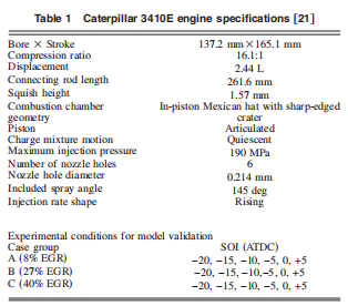
whose specifications are listed in Table 1. The gaseous emissions recorded in the experiments include NOx, intake CO2, exhaust CO2, carbon monoxide, and hydrocarbons. The particulate was measured using a full dilution tunnel and an AVL DPL 439 par- ticulate an alyzer. The EGR level was varied by changing the ex- haust back pressure. The intake and exhaust pressures were con- trolled by two Omega PID controllers, and the intake air flow rates were measured using critical flow orifices.
Experimental data obtained using a high-pressure injector [21] were simulated by the model. The engine operating conditions were optimized to achieve low NOx and particulate emissions and fuel consumption. The parameters that were varied included start- of-injection timing and EGR. The fuel injector was a production style Caterpillar electronic unit injector (EUI). The experimental results indicated that low emissions could be achieved by optimiz- ing the operating conditions to allow an optimal time interval between the end of fuel injection and the start of combustion. This is to allow a longer time for better mixing to produce a more homogeneous mixture. The experimental conditions used for model validation are also listed in Table 1 and include three EGR levels.
4 Results
4.1 Sandia Combustion Chamber. Experimental results of the Sandia combustion chamber [7,8] were used to validate the present models. The baseline experimental conditions for model validations are listed in Table 2.
The computations used a 0.5 deg sector mesh with 2 mm grid size in both radial and axial directions. The computational domain was 12.6 cm in diameter and 10 cm in height such that the total volume is the same as that of the combustion chamber in the experiment. Uniform chamber temperature, pressure, and species concentration based on experimental data were assumed initially without considering combustion radicals.
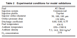
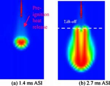
Fig. 1 Sample images of the predicted fuel spray and gas tem- perature distributions for dnozz =100 μm, Tamb =900 K, Pamb =138 MPa, pamb =14.8 kg/m3. Color scale: 900 to 2600 K.
A typical image of predicted fuel spray and gas temperature distributions of a free diesel lift-off flame is shown in Fig. 1. The injector is located at the top of the image. It can be seen that the liquid fuel undergoes atomization, vaporization, and mixing with entrained air before the lift-off location and then enters the reac- tion zones. Put into the context of a transient injection process, chemical reactions take place once the fuel is injected and mixed with air, and lead to autoignition at a certain location as seen in Fig. 1(a). Note that in Fig. 1(a), the light colors seen between the spray tip and the ignition location indicate a continuous tempera- ture rise as a result of preignition chemical reactions. The ignition location is approximately where the steady-state flame is stabi- lized in most cases, i.e., the lift-off location. The lift-off length is thus determined by both fluid mechanics and chemical kinetics that take place during the fuel/air mixing process prior to the lift-off location.
It is believed that chemical reactions prior to the lift-off loca- tion play an important role such that the flame is stabilized due to successive ignition events of the incoming fuel-air mixture. For example, it has been demonstrated that after the flame is estab- lished, if the chemical reactions before the lift-off location are suddenly deactivated, the flame is blown downstream and extin- guished. It is noted that the high gas velocity of the injected diesel fuel jet would require an unreasonably high turbulent flame speed to balance the incoming reactive mixture in order to stabilize a free standing diesel flame. Nonetheless, more research is needed to study the physics of diesel flame lift-off under engine conditions.
4.1. 1 Spatial Soot Distributions. Planar laser-induced incan- descence (PLII) images of soot along a thin plane of the fuel jet were compared with model predictions, as shown in Fig. 2. The injector orifice is located at the far left center of each image, with fuel being injected to the right. The flame lift-off length was de- termined from the OH chemiluminescence images in the experi- ments [7,8]. It is defined as the axial distance between the orifice and the location where the OH chemiluminescence intensity is approximately 50% of that just downstream of the initial rapid rise in the OH chemiluminescence. The cross-sectional average equivalence ratio at the flame lift-off length was estimated and is given on the left of the PLII images.
The present simulated soot mass fraction distributions are given in Fig. 2(b) to compare with the PLII images. The predicted lift- off length was determined from the contour of OH species using a similar method as in the experiments. The predicted equivalence ratio at the lift-off length is also given on the left of the images. The color scale of the predicted soot mass fraction is also shown in Fig. 2.
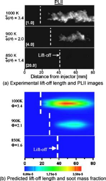
Fig. 2 Comparisons between PLII images and predicted soot mass fractions at the central plane of the fuel jet at 3.2 ms ASI. The equivalence ratios were estimated at the lift-off length. Relative PLII camera gain is given in brackets. dnozz =100 μm, Pinj =138 MPa, pamb =14.8 kg/m3.
It can be seen that the predicted soot distributions agree ex- tremely well with the experiments. Both experiments and simula- tions show that as the ambient gas temperature decreases, lift-off length increases, soot concentration decreases, and the equiva- lence ratio at the lift-off length also decreases. The conditions with ambient temperatures 1000 and 900 K are found to be soot- ing cases while no soot production is observed for the 850 K case, as revealed by both the experiments and simulations. In the simu- lations, the two sooting cases are found to have a soot mass frac- tion of the order of 1.0E _ 5 while the predicted maximum soot mass fraction is only about 1.0E _ 8 for the 850 K case. Other comparisons between model results and experimental images sug- gest that a soot mass fraction of 1.0E _ 5 can be used as the crite- rion to specify sooting and nonsooting conditions in the simula- tions. This criterion is used later in this paper to determine the sooting limit of injectors with different orifice diameters.
The temporal evolution of a typical injection and combustion event is illustrated in Fig. 3. Time after start of injection (ASI) for each image is given on the left. The distance from the injector is shown at the bottom. The dashed vertical line shows the lift-off length (18.3 mm) and the solid line shows the x= 50 mm position, which was found in the experiments to have the peak soot emis- sions at 3.2 ms ASI.
It can be seen from the figure that the evolution of the soot emissions predicted by the model agrees well with the experimen- tal results, especially after 2.0 ms. It was found that the model predicts a slightly longer ignition delay which can explain the lower soot formation at the early stages, e.g., at 1.3 ms ASI. Nu- merical results indicate that soot does not appear upstream of the lift-off length, which is consistent with the conclusion drawn from the experiments [8].
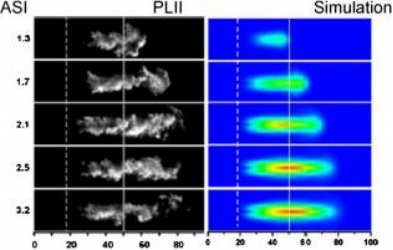
Fig. 3 Time sequence (ASI in ms) of PLII images and predicted soot mass fraction contours. The lift-off length and x=50 mm positions are shown on the images with vertical dashed and solid lines, respectively. dnozz =100 μm, Pinj =138 MPa, Tamb =1000 K, pamb =14.8 kg/m3.
4.1. 2 Axial Soot Distributions. The axial distributions of soot along the centerline of the fuel jet were also compared. Figure 4 shows comparisons of measured time-averaged KL factors and predicted soot mass fraction at 3.2 ms ASI. The KL factor is an indication of optical thickness derived from laser-extinction soot measurements [8]. The KL factor is proportional to the mass of soot along the line of sight of the extinction measurement, so it can be compared with the predicted soot mass that is integrated along the same line.
Optical thickness data were acquired at multiple axial locations along the centerline of the fuel jet at a certain time after start of injection. Due to the different nature of the KL factor from mea- surements and the integrated soot mass from the simulations, only qualitative comparisons can be made to assess the model perfor- mance. Thus, both measured KL factors and predicted soot mass are normalized to allow qualitative comparisons, as shown in Fig. 4.
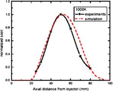
Fig. 4 Comparisons of measured time-averaged KL factors and predicted soot mass along the central axis of the fuel jet for the same conditions as in Fig. 3. Both measured and pre- dicted data were normalized to allow qualitative comparison. Results were acquired at 3.2 ms ASI for dnozz =100 μm, Tamb =1000 K, Pinj =138 MPa, pamb =14.8 kg/m3.
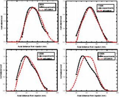
Fig. 5 Comparisons of measured time-averaged KL factors and predicted soot mass for various ambient temperatures 950, 1100, 1200, and 1300 K. Both measured and predicted data were normalized to allow qualitative comparison. Results were acquired at 3.2 ms ASI for dnozz =100 μm, Pinj =138 MPa, pamb =14.8 kg/m3.
Optical thickness data were acquired at multiple axial locations along the centerline of the fuel jet at a certain time after start of injection. Due to the different nature of the KL factor from mea- surements and the integrated soot mass from the simulations, only qualitative comparisons can be made to assess the model perfor- mance. Thus, both measured KL factors and predicted soot mass are normalized to allow qualitative comparisons, as shown in Fig. 4.
Comparisons of the normalized curves show good agreement in the general trend of the soot distribution along the jet central axis. Although the positions of the peak value of soot emissions differ slightly between the simulation and experiments (50 mm in ex- periments and ~55 mm in simulation), the agreement in the shape of the curves indicates that the transient features of soot formation and oxidation processes are captured by the present model.
Comparisons between the measured KL factors and predicted soot mass along the central axis at 3.2 ms ASI were also presented in Fig. 5 for other ambient gas temperature conditions of 950, 1100, 1200, and 1300 K. It can be seen that the predicted axial soot distributions agree with measurements very well. It can be seen that as the ambient temperature increases, the peak of the soot curve moves upstream toward the fuel jet. The early soot formation is consistent with the observation that lift-off length decreases at high ambient temperatures as in Fig. 2.
4.1. 3 Radial Soot Distribution. The measured radial soot dis- tribution 50 mm downstream of the injector (location indicated by the vertical solid lines in Fig. 3) was also compared with simula- tions in Fig. 6. Optical thickness data were acquired at multiple radial locations 50 mm from the injector at 3.2 ms ASI for the same conditions as in Fig. 3. Note that a 3-D cubic mesh with 2 mm grid size was used for the calculation such that it would be easier to integrate the soot mass in the radial direction. As before, both measured KL factors and predicted soot mass were normal- ized to allow qualitative comparisons. Figure 6 also indicates that the simulation results match the experiments very well even for such a s mall length scale (note that the length scale is 20 mm in the radial direction while it is 100 mm for the axial direction).
4.1.4 Sooting Tendency of Diesel Spray. The ultimate goal of the numerical model is to predict the sooting tendency of a diesel injector under different operating conditions. Figure 7 shows com- parisons of the measured and predicted sooting tendency of diesel injectors with different orifice diameters in an ambient density- temperature domain. To the left of each curve are the nonsooting regimes and to the right are sooting regimes. In the experiments, the sooting limit is determined by the visibility of soot in the PLII images. In the simulations, the maximum soot mass fraction of 1.0E _ 5 is used as the criterion, as discussed earlier.
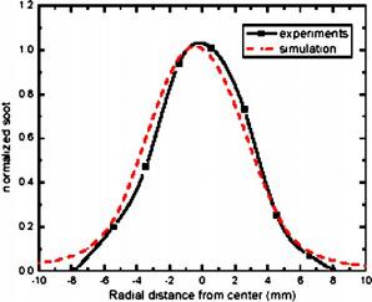
Fig. 6 Comparisons of measured time-averaged KL factors and predicted soot mass as a function of radial distance from the jet centerline at an axial distance of 50 mm from the orifice (vertical solid line in Fig. 3). Both measured and predicted data were normalized to allow qualitative comparison. Results were acquired at 3.2 ms ASI for the same conditions as in Fig. 3.
To determine the sooting limit in the simulation, cases of dif- ferent temperatures with a 25 K interval were simulated at a fixed ambient density. For example, nonsooting and sooting cases are marked with open and closed symbols, respectively, as shown in Fig. 7. The average temperature between adjacent nonsooting and sooting cases is regarded as the sooting limit for a specific injector at the corresponding ambient density condition.
As can be seen in Fig. 7, although there are discrepancies be- tween the exact locations of the measured and predicted sooting curves, especially for the s mall orifice (50 μm) injector, the trends are well predicted. As ambient density and temperature increase, or as orifice diameter increases, the sooting tendency increases. The discrepancy between measurements and predictions for the s mall orifice is probably due to the significant difference in the spray atomization and mixing processes between orifices with a conventional size and a s mall size which may not be well captured by the present spray model.
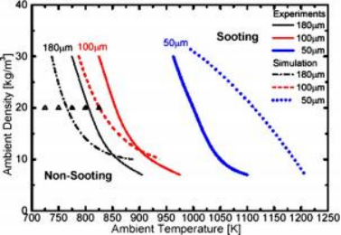
Fig. 7 Measured (solid lines) and predicted (dashed) sooting and nonsooting regimes as a function of ambient gas tempera- ture and density for Pinj =138 MPa. For the conditions of each curve, nonsooting combustion occurs to the left and sooting combustion to the right of each curve.
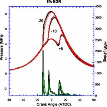
Fig. 8 Comparisons of measured (solid line) and predicted (dotted) cylinder pressure and heat release rate data for 8% EGR cases (SOI=−20, −10, and +5ATDC)
4.2 Caterpillar Diesel Engine. The present models were fur- ther applied to simulate combustion and emission processes in a heavy-duty diesel engine. Figures 8 and 9 show the measured and computed cylinder pressure and heat release rate data for selected cases. The model is seen to perform well over a wide range of engine conditions. The heat release rate data do not exhibit the distinct premixed and diffusion burn characteristics of conven- tional diesel engines. The highly premixed burned features of the present PCCI experiments are captured well by the model.
The predicted soot and NOx (i.e., sum of NO and NO2) emis- sions were also compared with the measurements, as shown in Figs. 10 and 11. It can be seen that the overall trends of soot and NOx are captured with respect to the start-of-injection timing. Dis- crepancies in soot emissions at early injection timings may be due to the details of the spray/wall interactions. It is of interest to note that engine-out soot emissions reach a peak value when fuel is injected near top-dead-center. The present model also predicts cor- rectly the soot reduction seen at further retarded injection timing (e.g., SOI= + 5ATDC) for all different EGR levels.
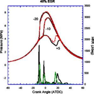
Fig. 9 Comparisons of measured (solid line) and predicted (dotted) cylinder pressure and heat release rate data for 40% EGR cases (SOI=−20, −10, and +5ATDC)
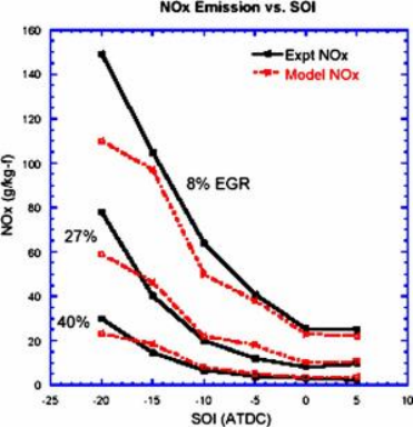
Fig. 10 Measured and predicted engine-out NOx emissions for cases listed in Table 1
The numerical model can explain the soot emission reduction seen as the injection is further retarded past TDC. This reduction is not seen in the conventional diesel combustion soot-NOx trade- off with respect to injection timing. Figure 12 shows the total in-cylinder soot mass evolutions for three different injection tim- ings, i.e., SOI= -10, 0, +5ATDC. The model results indicate that the lower exhaust soot emissions for SOI= -10ATDC are due to a better oxidation process as compared to that of SOI= 0ATDC. On the other hand, a lower soot emission for SOI= 5ATDC is because less soot is formed in the cylinder as a result of the low- temperature combustion (as also can be seen from the low cylin- der pressure in Figs. 8 and 9 for SOI= 5ATDC). The above low- temperature combustion characteristics are consistent with results in HSDI diesel engines [22] as well, and can be further facilitated to achieve low-emission diesel PCCI operation.
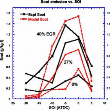
Fig. 11 Measured and predicted engine-out soot emissions for cases listed in Table 1
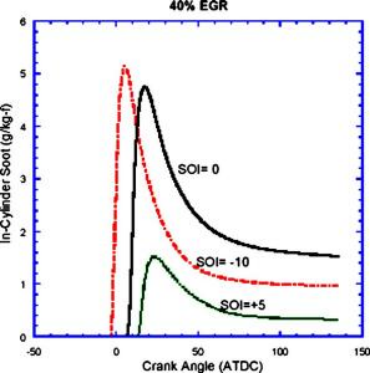
Fig. 12 In-cylinder soot mass histories for 40% EGR cases at three different injection timings. Values at exhaust valve open- ing (130 ATDC) are shown in Fig. 11.
5 Conclusions
A numerical model has been developed to simulate diesel fuel jet combustion in a combustion vessel and in a heavy-duty diesel engine. The model uses a skeletal reaction mechanis m to describe the fuel oxidation and NOx formation processes and a phenom- enological model to simulate soot formation and oxidation.
The model successfully predicts the lift-off length of a free diesel diffusion flame under various ambient conditions. The model results indicate that chemical reactions prior to the lift-off location are important for the stabilization of the lift-off flame. The simulations also agree with the measurements in predicting the sooting tendency of diesel fuel jets increases as the ambient gas density, temperature, or orifice diameter increases.
Experiments conducted in a heavy-duty diesel engine under PCCI-like conditions were also modeled. The predicted heat re- lease rate data, NOx, and soot emissions agreed well with the measurements. The model results indicate that low soot emissions can be obtained at late injection timings (i.e., SOI past TDC) by suppressing the total soot formation as a result of low-temperature combustion. Since NOx emissions decrease monotonically as in- jection is retarded, such a late injection scheme can be utilized for simultaneous soot and NOx reduction for future low-emission die- sel PCCI engines.
Acknowledgment
The authors acknowledge the financial support by the DOE/ Sandia National Labs and Caterpillar, Inc. Experimental data pro- vided by Dr. L. Pickett and Dr. D. Siebers (Sandia) and Adam Klingbeil and Jim von der Ehe (University of Wisconsin— Madison) for the model validation are greatly appreciated.
References
[1] Dec, J. E., 1997, “A Conceptual Model of DI Diesel Combustion Based on Laser Sheet Imaging,” SAE Paper No. 970873.
[2] Dec, J. E., and Canaan, R. E., 1998, “PLIF Imaging of NO Formation in a DI Diesel Engine,” SAE Paper No. 980147.
[3] Zhao, H., and Ladommatos, N., 1998, “Optical Diagnostics for Soot and Tem- perature Measurement in Diesel Engines,” Prog. Energy Combust. Sci., 24, pp. 221–255.
[4] Dec, J. E., and Tree, D. R., 2001, “Diffusion Flame/Wall Interactions in a Heavy-Duty Diesel Engine,” SAE Paper No. 2001-01-1295.
[5] Musculus, M. P., Dec, J. E., and Tree, D. R., 2002, “Effects of Fuel Parameters and Diffusion Flame Lift-Off on Soot Formation in a Heavy-Duty DI Diesel Engine,” SAE Paper No. 2002-01-0889.
[6] Bruneaux, G., Verhoeven, D., and Baritaud, T., 1999, “High-Pressure Diesel Spray and Combustion Visualization in a Transparent Model Diesel Engine,” SAE Paper No. 1999-01-3648.
[7] Pickett, L. M., and Siebers, D. L., 2004, “Non-Sooting, Low Flame Tempera- ture Mixing-Controlled DI Diesel Combustion,” SAE Paper No. 2004-01- 1399.
[8] Pickett, L. M., and Siebers, D. L., 2004, “Soot in Diesel Fuel Jets: Effects of Ambient Temperature, Ambient Density, and Injection Pressure,” Combust. Flame, 138, pp. 114–135.
[9] Hergart, C., Barths, H., and Peters, N., 1999, “Modeling the Combustion in a S mall-Bore Diesel Engine Using a Method Based on Representative Interac- tive Flamelets,” SAE Paper No. 1999-01-3550.
[10] Tao, F., Golovitchev, V. I., and Chomiak, J., 2004, “A Phenomenological Model for the Prediction of Soot Formation in Diesel Spray Combustion,” Combust. Flame, 136, pp. 270–282.
[11] Kong, S. C., and Reitz, R. D., 2002, “Application of Detailed Chemistry and CFD for Predicting Direct Injection HCCI Engine Combustion and Emis- sions,” Proc. Combust. Inst., 29, pp. 663–669.
[12] Kong, S. C., Patel, A., Yin, Q., and Reitz, R. D., 2003, “Numerical Modeling of Diesel Engine Combustion and Emissions Under HCCI-Like Conditions With High EGR Levels,” SAE Paper No. 2003-01-1087.
[13] Amsden, A. A., 1997, “KIVA-3V: A Block-Structured KIVA Program for En- gines with Vertical or Canted Valves,” LA-13313-MS.
[14] Han, Z., Uludogan, A., Hampson, G. J., and Reitz, R. D., 1996, “Mechanis m of Soot and NOx Emission Reduction Using Multiple-Injection in a Diesel Engine,” SAE Paper No. 960633.
[15] Patterson, M. A., and Reitz, R. D., 1998, “Modeling the Effects of Fuel Spray Characteristics on Diesel Engine Combustion and Emissions,” SAE Paper No. 980131.
[16] Han, Z., and Reitz, R. D., 1995, “Turbulence Modeling of Internal Combustion Engines Using RNG k-∈ Models,” Combust. Sci. Technol., 106, pp. 267–295.
[17] Kee, R. J., Rupley, F. M., and Miller, J. A., 1989, “CHEMKIN-II: A FOR- TRAN Chemical Kinetics Package for the Analyses of Gas Phase Chemical Kinetics,” Sandia Report, SAND 89-8009.
[18] Patel, A., Kong, S.-C., and Reitz, R. D., 2004, “Development and Validation of a Reduced Reaction Mechanis m for HCCI Engine Simulations,” SAE Paper No. 2004-01-0558.
[19] Golovitchev, V. I., 2000, http://www.tfd.chalmers.se/~valeri/MECH.html, Chalmers Univ of Tech, Goteborg, Sweden.
[20] S mith, G. P., Golden, D. M., Frenklach, M., Moriarty, N. W., Eiteneer, B., Goldenberg, M., Bowman, C. T., Hanson, R. K., Song, S., Gardiner, W. C., Lissianski, V. V., and Qin, Z., 2000, http://www.me.berkeley.edu/gri-mech/.
[21] Klingbeil, A. E., 2002, “Particulate and NOx Reduction in a Heavy-Duty Die- sel Engine Using High Levels of Exhaust Gas Recirculation and Very Early and Very Late Injection,” M.S. thesis, University of Wisconsin—Madison.
[22] Miles, P. C., Choi, D., Pickett, L. M., Singh, I. P., Henein, N., RempelEwert, B. A., Yun, H., and Reitz, R. D., 2004, “Rate-Limiting Processes in Late- Injection, Low-Temperature Diesel Combustion Regimes,” Proc. THIESEL 2004 Conference, pp. 429–447.
详细内容请见附件
免责声明:
本页面/内容部分素材来源于互联网公 开 信 息,旨在传递更多信息,不代表本平台立场。
版权归原作者或机构所有,如涉及侵权,请通过平台联系我们,我们将在核实后第一时间处理。
本平台对转载内容的真实性、准确性不作任何保证,用户需自行判断并承担使用风险。