从Butler-Volmer方程查看电荷转移阻抗的依赖关系

其中：    固相最大锂浓度，    固相表明锂浓度，    液相锂浓度，    电化学反应过电位，    阳极和阴极传递系数，    法拉第常数，    气体常数。

在COMSOL中，采用归一化参考交换电流密度    代替反应速率常数    ：

其中：    ,    。

   ，当    时，式（1）泰勒展开忽略高次项有：

有定义（基于面电阻    ）：

考虑多孔电极的活性面积    ，总电阻(    )：

那么通过EIS测试得到    可以反向计算出参考交换电流密度    

其中    ，假设活性材料颗粒为半径均一的球形颗粒，活性比表面积：    ，    :活性材料体积分数，    :活性材料半径。

根据式（8）,观察电荷转移阻抗的依赖关系:

(a).     ;

(b).     ;

(c).     ;

(d).      .

在    常规取值区间内，Rct单调递减。

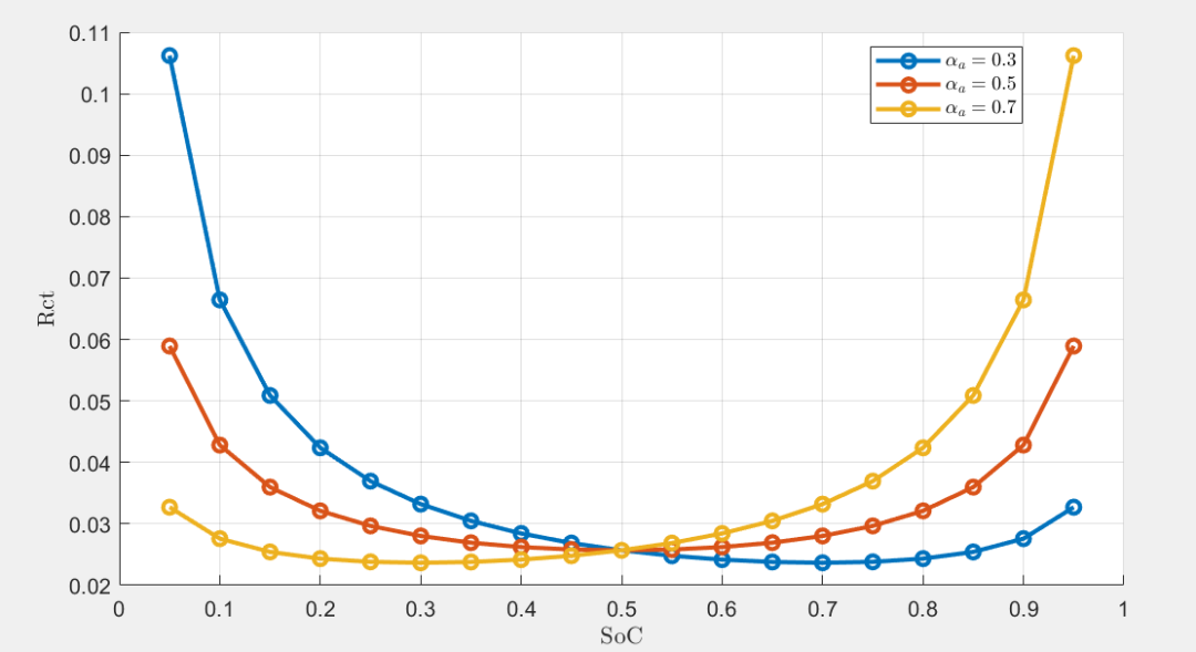
在    ，不同    下，Rct随SoC的变化如Fig1所示，其变化趋势与实测DCR相似，呈现两端高中间低的特点。

 

 

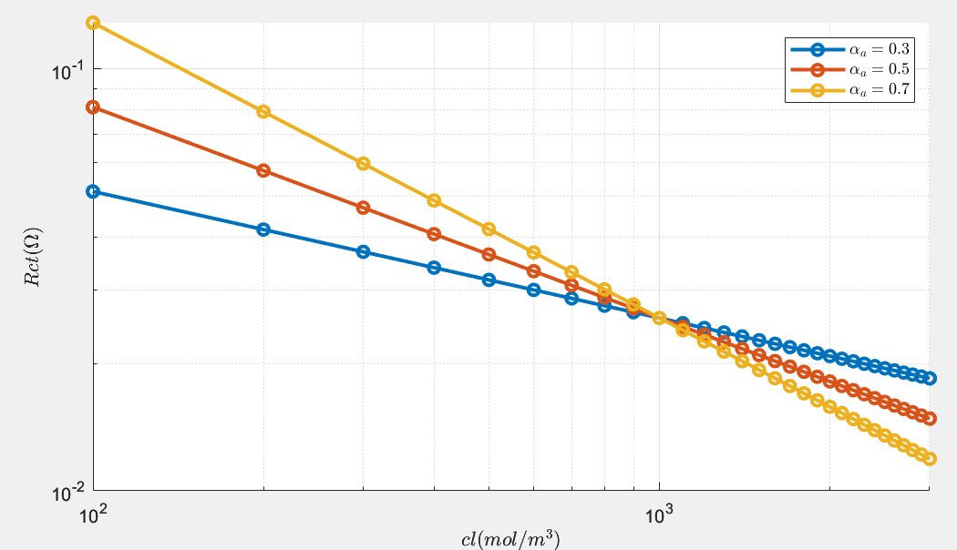
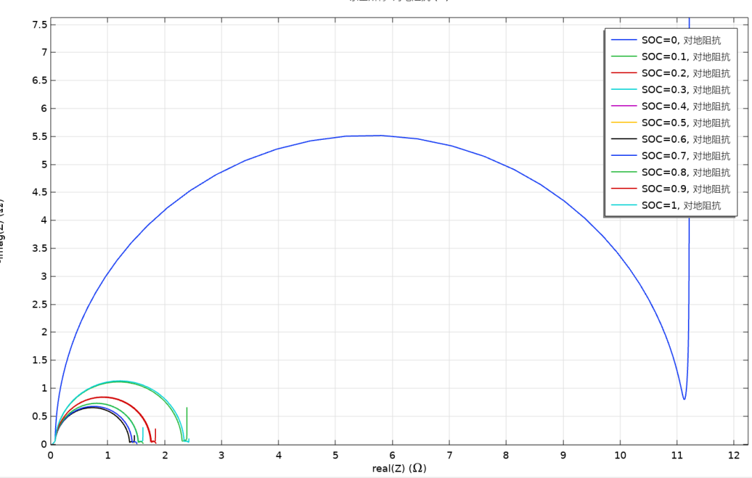
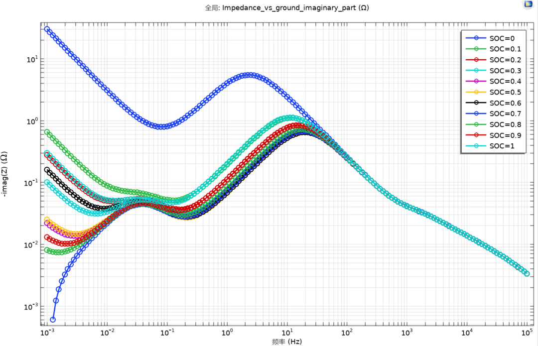
现采用COMSOL进行EIS测试模拟验证式（8）的依赖关系，不同SoC(全电池)下的负极的Nyquist和Bode图如Fig3-4所示：

 

 

根据Fig3-4提取Rct,按式（8）拟合结果如Fig5所示：

 

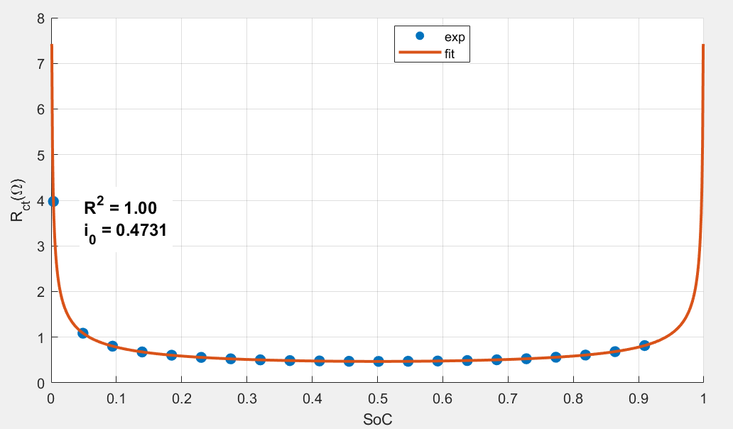
Matlab拟合代码：

sto=[0.0035
0.048786
0.094071
0.13936
0.18464
0.22993
0.27521
0.3205
0.36578
0.41107
0.45636
0.50164
0.54693
0.59221
0.6375
0.68278
0.72807
0.77335
0.81864
0.86393
0.90921];

Rct=[3.9746
1.0875
0.8036
0.6769
0.6055
0.5577
0.526
0.5035
0.4873
0.48
0.4717
0.4701
0.4721
0.4779
0.4883
0.5049
0.5278
0.5608
0.6084
0.6834
0.8165];

R = 8.314;       % 气体常数 J/(mol·K)
T = 318.15;      % 温度 K
alph = 0.5;      % 电荷转移系数
F = 96485;       % 法拉第常数 C/mol
Sa= 0.12343;
% 优化目标函数（残差平方和）
obj_fun = @(x) norm(R.*T./(2*x*F*Sa.*(sto.^0.5).*(1-sto).^0.5) - Rct);

% 初始猜测
x0 = [0.5];  % [I0]

% 优化选项
options = optimoptions('fminunc', ...
    'Algorithm', 'quasi-newton', ...
    'Display', 'iter', ...
    'MaxIterations', 1000, ...
    'MaxFunctionEvaluations', 2000);

% 执行优化
[x_opt, fval] = fminunc(obj_fun, x0, options);

% 计算拟合值
Rct_fit = R.*T./(2*x_opt*F*Sa.*(sto.^0.5).*(1-sto).^0.5);

% 拟合优度 R²
SS_res = sum((Rct - Rct_fit).^2);
SS_tot = sum((Rct - mean(Rct)).^2);
R_squared = 1 - SS_res / SS_tot;

% 绘图
figure
scatter(sto, Rct, 60, 'filled', DisplayName='exp');
hold on;
sto_fit = 0:0.001:1;
plot(sto_fit, R.*T./(2*x_opt*F*Sa.*(sto_fit.^0.5).*(1-sto_fit).^0.5), '-', ...
    LineWidth=2, DisplayName='fit');
grid on;
legend('Location', 'best');
xlabel('SoC'); ylabel('R_{ct}');

text(0.05, max(Rct)*0.9, {sprintf('R^2 = %.2f', R_squared), sprintf('i_0 = %.4f', x_opt)}, ...
    'FontSize', 12, 'FontWeight', 'bold', 'BackgroundColor', 'w');

Ref:

DOI 10.1149/1945-7111/acf161