矩形薄板的有限元分析C++编程实现

采用4节点板单元建立受弯薄板的二维有限元模型,能量原理推导出基尔霍夫板的刚度和弯矩的二重积分表达式,利用高斯积分法得到单元刚度矩阵和弯矩的典型表达式。组装出矩阵位移法的整体刚度矩阵,通过罚函数法处理边界条件,得到有限元方程。 采用C++语言实现算法设计。将整体刚度矩阵(稀疏矩阵)进行Cholesky分解后存储于一维向量空间,求解有限元方程,得到各单元节点的位移向量,回代得到各单元板中心的弯矩值。使用该程序计算薄板受弯问题,结果符合预期。 关键词:基尔霍夫板(Kirchhoff–Love),二维弹性薄板,有限单元法(FEM),能量原理,应变能,形函数,二阶偏导,高斯积分,C++编程。 |
1. 引言
前面6篇文章采用矩阵位移法:通过2节点梁-杆单元分析连续多跨梁、弹性地基梁、平面/空间桁架及框架结构。矩阵位移法方法是有限单元法(FEM)的特例,有助于理解有限元法的基本思想。实际工程中除了一维弹性单元,还有二维/三维连续介质实体。
本文将采用“真正意义上”的有限单元法,在梁-杆单元分析模型的基础上,对程序进行了如下改进,使之适用于薄板弯曲问题。
输入x/y方向的单元数nxe/nye和单元尺寸aa/bb,
新增函数mesh_size()自动生成单元数nels和节点数nn,
新增函数geom_rect()自动生成节点坐标coord和节点编号num;输入单元类型element、积分节点数nip、维数ndim,
新增函数sample()生成高斯积分点的局部坐标s和加权系数wt;
新增函数fmplat()生成形函数关于高斯积分点的二阶偏导d2x、d2y、d2xy。
2. 矩形薄板的弹性分析
当板厚与中面特征尺寸(边长或直径)之比小于1/5时,可以按薄板计算。在侧向荷载作用下,薄板将产生弯曲变形,当板的最大弯曲挠度远小于板厚时,称为薄板小挠度问题。
2.1. 基尔霍夫板(Kirchhoff–Love)
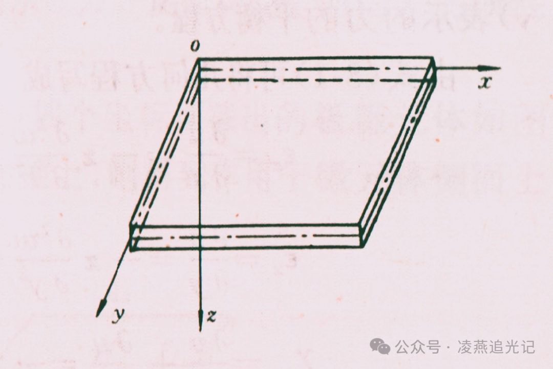
图1:薄板
当板厚与中面特征尺寸(边长或直径)之比远小于1时,可以采用基尔霍夫板假定:
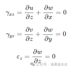


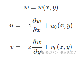
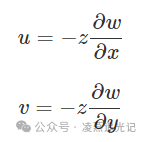
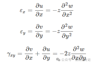
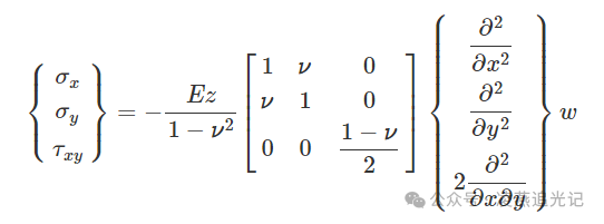
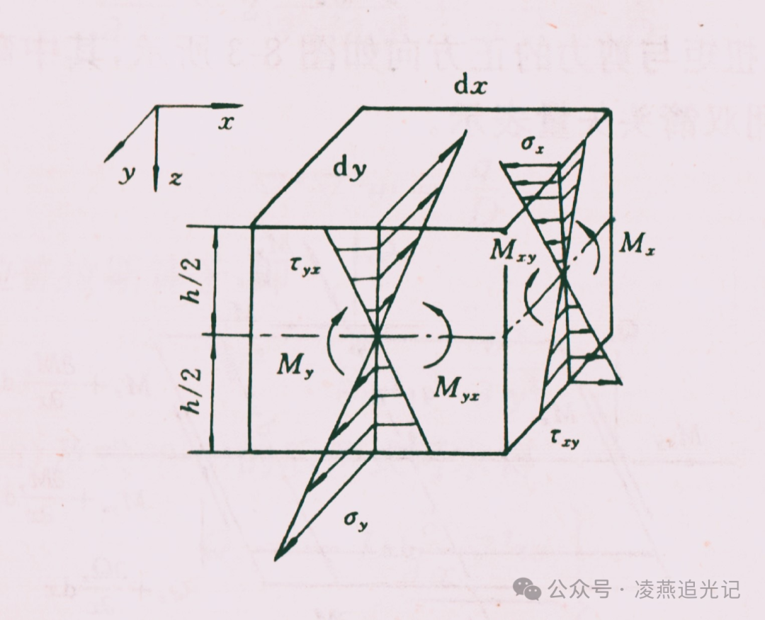
图2:板微元体
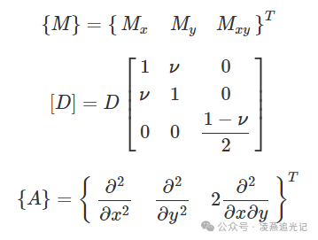
如上图所示,作用于微元体侧面上的内力矩为:
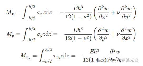
也可以写成矩阵形式:
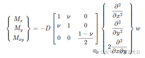
上式中,D为板的抗弯刚度,表达式为:
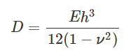
也可以写成:
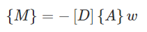
其中:
2.2. 高斯积分
由于矩形薄板是连续体,其内力与变形都是沿板面连续分布的。为了方便计算,采用高斯积分法,根据实际需求,选取合理数量(n个)的采样点(高斯点),将空间内连续分布的物理量(刚度、质量、内力、变形等)表示为n个高斯点与n个权系数的乘积之和,得到满足精度要求的结果。
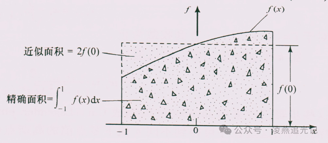
图3:一点高斯积分
如图3所示,高斯点为(0),权系数为2,即:
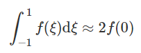
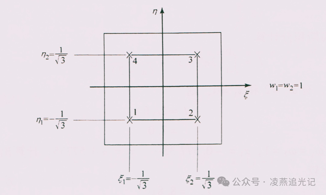
图4:二维2×2阶高斯积分
如图4所示,高斯点1、2、3、4的权系数均为1,即:
本文采用4×4也就是16个高斯积分点,直接参考数学界的科研成果,定义函数 sample() 生成各积分点局部坐标和加权系数,源码如下:
//This subroutine returns the local coordinates and weighting coefficients//of the integrating points.//输入:单元类型element, 单元的积分节点数nip, 维数ndim//输出:局部坐标s, 加权系数wt#include <string>#include <vector>#include <iostream>#include <utility>using namespace std;pair<vector<vector<double> >, vector<double> > sample(string element, int nip, int ndim) {double root3 = 1.0 / sqrt(3.0);double r15 = 0.2 * sqrt(15.0);vector<double> wt(nip);vector<vector<double> > s(nip, vector<double>(ndim));vector<double> w = {5.0 / 9.0, 8.0 / 9.0, 5.0 / 9.0};vector<double> v(9);for (int i = 0; i < 3; i++) {for (int j = 0; j < 3; j++) {int k = i * 3 + j;v[k] = w[i] * w[j];}}if (element == "line") ;else if (element == "triangle") ;else if (element == "quadrilateral") {switch (nip) {case 1:s[0][0] = 0.0;s[0][1] = 0.0;wt[0] = 4.0;break;case 4:s[0][0] = -root3;s[0][1] = root3;s[1][0] = root3;s[1][1] = root3;s[2][0] = -root3;s[2][1] = -root3;s[3][0] = root3;s[3][1] = -root3;fill(wt.begin(), wt.end(), 1.0);break;case 9:s[0][0] = -r15;s[0][1] = r15;s[1][0] = 0.0;s[1][1] = r15;s[2][0] = r15;s[2][1] = r15;s[3][0] = -r15;s[3][1] = 0.0;s[4][0] = 0.0;s[4][1] = 0.0;s[5][0] = r15;s[5][1] = 0.0;s[6][0] = -r15;s[6][1] = -r15;s[7][0] = 0.0;s[7][1] = -r15;s[8][0] = r15;s[8][1] = -r15;wt = v;break;case 16:s[0][0] = -0.861136311594053;s[0][1] = 0.861136311594053;s[1][0] = -0.339981043584856;s[1][1] = s[0][1];s[2][0] = 0.339981043584856;s[2][1] = s[0][1];s[3][0] = 0.861136311594053;s[3][1] = s[0][1];s[4][0] = s[0][0];s[4][1] = 0.339981043584856;s[5][0] = s[1][0];s[5][1] = s[4][1];s[6][0] = s[2][0];s[6][1] = s[4][1];s[7][0] = s[3][0];s[7][1] = s[4][1];s[8][0] = s[0][0];s[8][1] = -0.339981043584856;s[9][0] = s[1][0];s[9][1] = s[8][1];s[10][0] = s[2][0];s[10][1] = s[8][1];s[11][0] = s[3][0];s[11][1] = s[8][1];s[12][0] = s[0][0];s[12][1] = -0.861136311594053;s[13][0] = s[1][0];s[13][1] = s[12][1];s[14][0] = s[2][0];s[14][1] = s[12][1];s[15][0] = s[3][0];s[15][1] = s[12][1];wt[0] = 0.121002993285602;wt[1] = 0.226851851851852;wt[2] = wt[1];wt[3] = wt[0];wt[4] = wt[1];wt[5] = 0.425293303010694;wt[6] = wt[5];wt[7] = wt[1];wt[8] = wt[1];wt[9] = wt[5];wt[10] = wt[5];wt[11] = wt[1];wt[12] = wt[0];wt[13] = wt[1];wt[14] = wt[1];wt[15] = wt[0];break;case 25:s[0][0] = 0.906179845938664;s[0][1] = 0.906179845938664;s[1][0] = 0.538469310105683;s[1][1] = s[0][1];s[2][0] = 0.0;s[2][1] = s[0][1];s[3][0] = -0.538469310105683;s[3][1] = s[0][1];s[4][0] = -0.906179845938664;s[4][1] = s[0][1];s[5][0] = s[0][0];s[5][1] = 0.538469310105683;s[6][0] = s[1][0];s[6][1] = s[5][1];s[7][0] = 0.0;s[7][1] = s[5][1];s[8][0] = s[3][0];s[8][1] = s[5][1];s[9][0] = s[4][0];s[9][1] = s[5][1];s[10][0] = s[0][0];s[10][1] = 0.0;s[11][0] = s[1][0];s[11][1] = 0.0;s[12][0] = 0.0;s[12][1] = 0.0;s[13][0] = s[3][0];s[13][1] = 0.0;s[14][0] = s[4][0];s[14][1] = 0.0;s[15][0] = s[0][0];s[15][1] = -0.538469310105683;s[16][0] = s[1][0];s[16][1] = s[15][1];s[17][0] = 0.0;s[17][1] = s[15][1];s[18][0] = s[3][0];s[18][1] = s[15][1];s[19][0] = s[4][0];s[19][1] = s[15][1];s[20][0] = s[0][0];s[20][1] = -0.906179845938664;s[21][0] = s[1][0];s[21][1] = s[20][1];s[22][0] = 0.0;s[22][1] = s[20][1];s[23][0] = s[3][0];s[23][1] = s[20][1];s[24][0] = s[4][0];s[24][1] = s[20][1];wt[0] = 0.056134348862429;wt[1] = 0.113400000000000;wt[2] = 0.134785072387521;wt[3] = 0.113400000000000;wt[4] = 0.056134348862429;wt[5] = 0.113400000000000;wt[6] = 0.229085404223991;wt[7] = 0.272286532550750;wt[8] = 0.229085404223991;wt[9] = 0.113400000000000;wt[10] = 0.134785072387521;wt[11] = 0.272286532550750;wt[12] = 0.323634567901235;wt[13] = 0.272286532550750;wt[14] = 0.134785072387521;wt[15] = 0.113400000000000;wt[16] = 0.229085404223991;wt[17] = 0.272286532550750;wt[18] = 0.229085404223991;wt[19] = 0.113400000000000;wt[20] = 0.056134348862429;wt[21] = 0.113400000000000;wt[22] = 0.134785072387521;wt[23] = 0.113400000000000;wt[24] = 0.056134348862429;break;default:cout << "Wrong number of integrating points for a quadrilateral" << endl;break;}}else if (element == "tetrahedron");else if (element == "hexahedron");elsecout << "Not a valid element type" << endl;return make_pair(s, wt);}
2.3. 形函数与二阶偏导
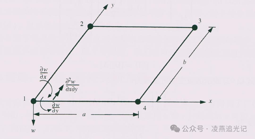
图5:矩形板弯曲单元
如上图所示矩形单元,假设每个节点有4个自由度:

单元自由度可以定义为:

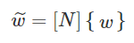
参照《弹性梁的几何非线性有限元分析C++编程实现》第2.1节,连续变量w可以根据离散后的节点值确定,即表示为单元4个节点形函数与节点4个自由度的乘积之和:

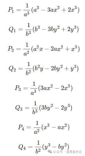
则形函数依次表示为:
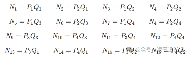
相应的二阶偏导:(i,j=1,2,3,4 以及 k=1,2,3,…16)
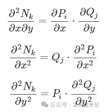
//This subroutine forms the 2nd derivatives for rectangular plate bending elements.//输入:单元积分点坐标points, x方向单元尺寸aa, y方向单元尺寸bb, 单元积分点编号ii//输出:关于ξ形函数的二阶偏导d2x, 关于η形函数的二阶偏导d2y, 关于ξ和η形函数的混合二阶偏导d2xy#include <tuple>#include <vector>using namespace std;tuple<vector<float>, vector<float>, vector<float> >fmplat(vector<vector<double> > points, float aa, float bb, int ii, int ndof) {float x, e, xp1, xp12, xp13, ep1, ep12, ep13, p1, q1, p2, q2, p3, q3, p4, q4;float dp1, dq1, dp2, dq2, dp3, dq3, dp4, dq4, d2p1, d2p2, d2p3, d2p4, d2q1, d2q2, d2q3, d2q4;vector<float> d2x(ndof);vector<float> d2y(ndof);vector<float> d2xy(ndof);x = points[ii][0];e = points[ii][1];xp1 = x + 1.0;xp12 = xp1 * xp1;xp13 = xp12 * xp1;ep1 = e + 1.0;ep12 = ep1 * ep1;ep13 = ep12 * ep1;p1 = 1.0 - 0.75 * xp12 + 0.25 * xp13;q1 = 1.0 - 0.75 * ep12 + 0.25 * ep13;p2 = 0.5 * aa * xp1 * (1.0 - xp1 + 0.25 * xp12);q2 = 0.5 * bb * ep1 * (1.0 - ep1 + 0.25 * ep12);p3 = 0.25 * xp12 * (3.0 - xp1);q3 = 0.25 * ep12 * (3.0 - ep1);p4 = 0.25 * aa * xp12 * (0.5 * xp1 - 1.0);q4 = 0.25 * bb * ep12 * (0.5 * ep1 - 1.0);dp1 = 1.5 * xp1 * (0.5 * xp1 - 1.0);dq1 = 1.5 * ep1 * (0.5 * ep1 - 1.0);dp2 = aa * (0.5 - xp1 + 0.375 * xp12);dq2 = bb * (0.5 - ep1 + 0.375 * ep12);dp3 = 1.5 * xp1 * (1.0 - 0.5 * xp1);dq3 = 1.5 * ep1 * (1.0 - 0.5 * ep1);dp4 = 0.5 * aa * xp1 * (0.75 * xp1 - 1.0);dq4 = 0.5 * bb * ep1 * (0.75 * ep1 - 1.0);d2p1 = 1.5 * x;d2p2 = 0.25 * aa * (3.0 * x - 1.0);d2p3 = -d2p1;d2p4 = 0.25 * aa * (3.0 * x + 1.0);d2q1 = 1.5 * e;d2q2 = 0.25 * bb * (3.0 * e - 1.0);d2q3 = -d2q1;d2q4 = 0.25 * bb * (3.0 * e + 1.0);d2x[0] = d2p1 * q1;d2x[1] = d2p2 * q1;d2x[2] = d2p1 * q2;d2x[3] = d2p2 * q2;d2x[4] = d2p1 * q3;d2x[5] = d2p2 * q3;d2x[6] = d2p1 * q4;d2x[7] = d2p2 * q4;d2x[8] = d2p3 * q3;d2x[9] = d2p4 * q3;d2x[10] = d2p3 * q4;d2x[11] = d2p4 * q4;d2x[12] = d2p3 * q1;d2x[13] = d2p4 * q1;d2x[14] = d2p3 * q2;d2x[15] = d2p4 * q2;d2y[0] = p1 * d2q1;d2y[1] = p2 * d2q1;d2y[2] = p1 * d2q2;d2y[3] = p2 * d2q2;d2y[4] = p1 * d2q3;d2y[5] = p2 * d2q3;d2y[6] = p1 * d2q4;d2y[7] = p2 * d2q4;d2y[8] = p3 * d2q3;d2y[9] = p4 * d2q3;d2y[10] = p3 * d2q4;d2y[11] = p4 * d2q4;d2y[12] = p3 * d2q1;d2y[13] = p4 * d2q1;d2y[14] = p3 * d2q2;d2y[15] = p4 * d2q2;d2xy[0] = dp1 * dq1;d2xy[1] = dp2 * dq1;d2xy[2] = dp1 * dq2;d2xy[3] = dp2 * dq2;d2xy[4] = dp1 * dq3;d2xy[5] = dp2 * dq3;d2xy[6] = dp1 * dq4;d2xy[7] = dp2 * dq4;d2xy[8] = dp3 * dq3;d2xy[9] = dp4 * dq3;d2xy[10] = dp3 * dq4;d2xy[11] = dp4 * dq4;d2xy[12] = dp3 * dq1;d2xy[13] = dp4 * dq1;d2xy[14] = dp3 * dq2;d2xy[15] = dp4 * dq2;return make_tuple(d2x, d2y, d2xy);}
2.4. 能量原理与刚度矩阵
根据能量原理,受弯板的应变能密度为:

将基尔霍夫板几何方程代入上式,积分得到应变能:

也可以写成:

上式即为受弯板的应变能表达式,可以写成如下形式(D和A表达式详本文2.1节):

其刚度矩阵为:
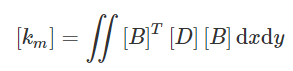
其中[B] = {A}[N],形函数N的表达式参照本文2.3节。
一个典型的刚度矩阵的元素表达式:

然后将单元刚度矩阵集结成整体刚度矩阵,并叠加到整体荷载向量,采用罚函数法处理边界条件,生成整体结构的有限元方程。程序自动求解有限元方程,得到总体 位移向量。
继续采用高斯积分法的思想,将计算结果(总体 位移向量)回代到本文2.1节的弯矩表达式,即可得到各单元中心处的弯矩值。这里需要重置高斯积分点nip=1来找到各单元板的中心点。
3. 程序设计(C++)
3.1. 网格划分
自动生成平面网格。具体分两步:
定义函数mesh_size(),根据指定单元类型element、单元节点数nod、各方向单元数nxe / nye / nze,生成单元数nels、节点数nn; 定义函数geom_rect(),根据上一步生成的单元数nels和节点数nn,生成各单元的节点坐标coord和节点编号num。
mesh_size() 和 geom_rect() 如下:
//This subroutine returns the number of elements (nels)//and the numberof nodes (nn) in a 2-d geometry-created mesh.//输入:单元类型element, 单元节点数nod, x、y、z向的单元数nxe、nye、nze//输出:单元数nels, 节点数nn#include <string>#include <utility>using namespace std;pair<int, int> mesh_size(string element, int nod, int nxe, int nye, int nze) {int nels, nn;if (element == "triangle") {nels = nxe * nye * 2;if (nod == 3)nn = (nxe + 1) * (nye + 1);if (nod == 6)nn = (2 * nxe + 1) * (2 * nye + 1);if (nod == 10)nn = (3 * nxe + 1) * (3 * nye + 1);if (nod == 15)nn = (4 * nxe + 1) * (4 * nye + 1);}else if (element == "quadrilateral") {nels = nxe * nye;if (nod == 4)nn = (nxe + 1) * (nye + 1);if (nod == 5)nn = (nxe + 1) * (nye + 1) + nxe * nye;if (nod == 8)nn = (2 * nxe + 1) * (nye + 1) + (nxe + 1) * nye;if (nod == 9)nn = (2 * nxe + 1) * (2 * nye + 1);}else if (element == "hexahedron") {nels = nxe * nye * nze;if (nod == 8)nn = (nxe + 1) * (nye + 1) * (nze + 1);if (nod == 14)nn = 4 * nxe * nye * nze + 2 * (nxe * nye + nye * nze + nze * nxe) + nxe + nye + nze + 1;if (nod == 20)nn = ((2 * nxe + 1) * (nze + 1) + (nxe + 1) * nze) * (nye + 1) + (nxe + 1) * (nze + 1) * nye;}return make_pair(nels, nn);}
//This subroutine forms the coordinates and connectivity for//a rectangular mesh of rt. angled triangular elements (3, 6, 10 or 15-node)//or quadrilateral elements (4, 8 or 9-node) counting in the x- or y-dir.//输入:单元类型element, 单元编号iel, 单元节点数nod, 节点编号方向dir,// 网格排列的x、y方向坐标x_coords、y_coords//输出:单元节点坐标coord, 单元节点编号向量num#include <string>#include <utility>#include <vector>#include <iostream>using namespace std;pair<vector<vector<float> >, vector<int> >geom_rect(string element, int iel, int nod, char dir,vector<float> x_coords, vector<float> y_coords) {int ip, iq, jel, fac1, nxe, nye;nxe = x_coords.size() - 1;vector<int> num(nod);vector<vector<float> > coord(nod, vector<float>(2));if (element == "triangle") ;if (element == "quadrilateral") {nye = y_coords.size() - 1;if (dir == 'x' || dir == 'r') {iq = iel / nxe + 1;ip = iel - (iq - 1) * nxe + 1;}else {ip = iel / nye + 1;iq = iel - (ip - 1) * nye + 1;}switch (nod) {case 4:if (dir == 'x' || dir == 'r') {num[0] = iq * (nxe + 1) + ip;num[1] = (iq - 1) * (nxe + 1) + ip;num[2] = num[1] + 1;num[3] = num[0] + 1;}else {num[0] = (ip - 1) * (nye + 1) + iq + 1;num[1] = num[0] - 1;num[2] = ip * (nye + 1) + iq;num[3] = num[2] + 1;}coord[0][0] = x_coords[ip - 1];coord[1][0] = x_coords[ip - 1];coord[2][0] = x_coords[ip];coord[3][0] = x_coords[ip];coord[0][1] = y_coords[iq];coord[1][1] = y_coords[iq - 1];coord[2][1] = y_coords[iq - 1];coord[3][1] = y_coords[iq];break;case 5:case 8:case 9:break;defalt:cout << "Wrong number of nodes for quadrilateral element" << endl;break;}}return make_pair(coord, num);}
3.2. 主程序流程图及C++源码
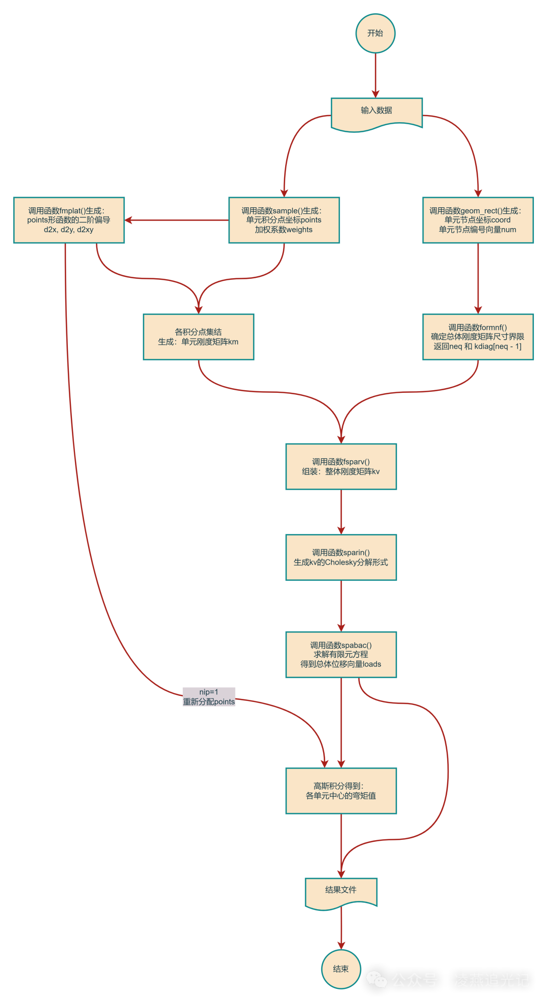
图6:主程序流程图
//===========================================================================// Program NO.7 Analysis of plates using 4-node rectangular plate elements.// Homogeneous material with identical elements.// Mesh numbered in x- or y- direction.//===========================================================================#include "geom.h"#include "main.h"#include <fstream>#include <iomanip>#include <iostream>#include <string>#include <tuple>#include <utility>#include <vector>using namespace std;int main() {int fixed_freedoms; //固定位移的数量int loaded_nodes; //受载节点数int ndim = 2; //维数int ndof = 16; //每个单元的自由度int nels; //单元数int neq; //网格自由度int nip = 16; //每个单元的积分节点数int nn; //节点数int nod = 4; //每个单元的节点数int nodof = 4; //每个节点的自由度int nprops = 2; //材料特性数int np_types; //不同材料的类型数目int nr; //约束节点数int nxe, nye; //x方向、y方向的单元数float aa, bb; //x方向、y方向单元尺寸float d; //板的弯曲刚度float e, v; //弹性模量, 泊松比float penalty = 1.0e20; //罚因子float th; //板的厚度pair<string, string> argv; //文件名返回值string fin_name, fout_name; //读入文件名,写出文件名string element = "quadrilateral"; //单元类型//========================= input and initialisation =========================argv = getname();fin_name = argv.first;ifstream fin(fin_name, ios::in);fout_name = argv.second;ofstream fout(fout_name, ios::out);fin >> nxe >> nye >> np_types; //从文件中读入: 单元行数和列数, 不同材料的类型数目fin >> aa >> bb >> th; //从文件中读入: x方向、y方向单元尺寸, 板的厚度auto result0 = mesh_size(element, nod, nxe, nye, 0); //返回:单元数, 节点数nels = result0.first;nn = result0.second;vector<float> bm(3); //弯矩向量(3个)vector<float> d2x(ndof); //关于ξ形函数的二阶偏导(单元的自由度)vector<float> d2y(ndof); //关于η形函数的二阶偏导(单元的自由度)vector<float> d2xy(ndof); //关于ξ和η形函数的混合二阶偏导(单元的自由度)vector<int> etype(nels); //单元特性类型向量(单元数)vector<int> g(ndof); //单元定位向量(单元的自由度)vector<int> num(nod); //单元节点编号向量(单元节点数目)vector<double> weights(nip); //数值积分加权系数(单元积分节点数)vector<float> x_coords(nxe + 1); //网格排列的x方向坐标(单元行数 + 1)vector<float> y_coords(nye + 1); //网格排列的x方向坐标(单元列数 + 1)vector<vector<float> > coord(nod, vector<float>(ndim)); //单元节点坐标(每个单元的节点数, 维数)vector<vector<float> > dtd(ndof, vector<float>(ndof)); //km的积分点矩阵(单元自由度, 单元自由度)vector<vector<float> > g_coord(nn, vector<float>(ndim)); //所有单元的节点坐标(节点数, 维数)vector<vector<int> > g_g(nels, vector<int>(ndof)); //总单元定位矩阵(单元数,每个单元的自由度)vector<vector<int> > g_num(nels, vector<int>(nod)); //总单元节点编号矩阵(单元数, 每个单元的节点数)vector<vector<float> > km(ndof, vector<float>(ndof)); //单元刚度矩阵(单元自由度, 单元自由度)vector<vector<int> > nf(nn, vector<int>(nodof, 1)); //节点自由度矩阵(节点数,每个节点的自由度数目)vector<vector<double> > points(nip, vector<double>(ndim)); //单元积分点坐标(每个单元的积分点数, 维数)vector<vector<float> > prop(np_types, vector<float>(nprops)); //单元特征矩阵(不同材料的类型数目, 材料特性数)for (int i = 0; i < np_types; i++) { //从文件中读入:单元特征矩阵for (int j = 0; j < nprops; j++)fin >> prop[i][j];}if (np_types > 1) { //从文件中读入:单元特性类型向量for (int i = 0; i < nels; i++)fin >> etype[i];}for (int i = 0; i <= nxe; i++) //生成:网格排列的x方向坐标x_coords[i] = i * aa;for (int j = 0; j <= nye; j++) //生成:网格排列的y方向坐标y_coords[j] = j * bb;fin >> nr; //从文件中读入:约束节点数vector<int> k1(nr); //约束节点编号向量(约束节点数)if (nr > 0) { //从文件中读入:约束节点编号及自由度for (int i = 0; i < nr; i++) {fin >> k1[i];for (int j = 0; j < nodof; j++) {int m = k1[i] - 1;fin >> nf[m][j];}}}auto result1 = formnf(nf);neq = result1.first; //返回:网格自由度数目nf = result1.second; //生成:节点自由度矩阵vector<int> kdiag(neq); //对角项局部向量(网格自由度数目)vector<float> loads(neq); //总体荷载/位移向量(网格自由度数目)//=============== loop the elements to find global array sizes ===============for (int i = 0; i < nels; i++) {auto result2 = geom_rect(element, i, nod, 'x', x_coords, y_coords);coord = result2.first; //单元节点坐标矩阵num = result2.second; //单元节点编号向量g = num_to_g(num, nf); //单元定位向量kdiag = fkdiag(g, kdiag); //对角项局部向量g_num[i] = num; //第i个单元的节点编号向量for (int j = 0; j < nod; j++) {int k = num[j] - 1;g_coord[k] = coord[j]; //第i个单元的节点坐标矩阵}g_g[i] = g; //第i个单元的定位向量}//mesh(g_coord, g_num, fin_name); //生成:初始网格的附录图(*.mesh)for (int i = 1; i < neq; i++) //生成:对角项局部向量kdiag[i] = kdiag[i] + kdiag[i - 1];fout << "There are " << neq << " equations and the skyline storage is "<< kdiag[neq - 1] << endl;cout << "There are " << neq << " equations and the skyline storage is "<< kdiag[neq - 1] << endl;//================ element stiffness integration and assembly ================vector<float> kv(kdiag[neq - 1]); //初始化:整体刚度向量auto result3 = sample(element, nip, ndim);//生成:单元积分点坐标,加权系数points = result3.first;weights = result3.second;for (int i = 0; i < nels; i++) {if (np_types > 1) {int m = etype[i] - 1;e = prop[m][0];v = prop[m][1];}else{e = prop[0][0];v = prop[0][1];}d = e * pow(th, 3) / (12.0 * (1.0 - pow(v, 2)));g = g_g[i];fill(km.begin(), km.end(), vector<float>(ndof, 0.0));for (int j = 0; j < nip; j++) {auto result4 = fmplat(points, aa, bb, j, ndof);d2x = get<0>(result4);d2y = get<1>(result4);d2xy = get<2>(result4);for (int k1 = 0; k1 < ndof; k1++) {for (int k2 = 0; k2 < ndof; k2++) {dtd[k1][k2] = 4.0 * aa * bb * d * weights[j] *(d2x[k1] * d2x[k2] / pow(aa, 4) + d2y[k1] * d2y[k2] / pow(bb, 4)+ (v * d2x[k1] * d2y[k2] + v * d2x[k2] * d2y[k1]+ 2.0 * (1.0 - v) * d2xy[k1] * d2xy[k2]) / (pow(aa, 2) * pow(bb, 2)));km[k1][k2] += dtd[k1][k2];}}}kv = fsparv(km, g, kdiag, kv); //生成:整体刚度矩阵}//===================== read loads and /or displacements =====================fin >> loaded_nodes; //受载节点数vector<int> k2(loaded_nodes); //受载节点编号向量if (loaded_nodes) {for (int i = 0; i < loaded_nodes; i++) {fin >> k2[i];int m1 = k2[i] - 1;for (int j = 0; j < nodof; j++) {if (nf[m1][j]) {int m2 = nf[m1][j] - 1;fin >> loads[m2];}}}}fin >> fixed_freedoms; //固定位移的数量vector<int> node(fixed_freedoms); //固定节点向量vector<int> no(fixed_freedoms); //固定自由度编号向量vector<int> sense(fixed_freedoms); //固定自由度的检测向量vector<float> value(fixed_freedoms); //给定位移向量if (fixed_freedoms) {for (int i = 0; i < fixed_freedoms; i++) {fin >> node[i] >> sense[i] >> value[i];int j = node[i] - 1;int k = sense[i] - 1;no[i] = nf[j][k];int m = no[i] - 1;int n = kdiag[m] - 1;kv[n] += penalty;loads[m] = kv[n] * value[i];}}kv = sparin(kv, kdiag); //整体刚度矩阵kv的Cholesky三角分解形式loads = spabac(kv, loads, kdiag); //求解有限元方程,得到总体 位移向量fout << endl << " Node Disp Rot-x Rot-y Twist-xy" << endl;cout << endl << " Node Disp Rot-x Rot-y Twist-xy" << endl;for (int i = 0; i < nn; i++) {fout << setw(4) << i + 1;cout << setw(4) << i + 1;for (int j = 0; j < nodof; j++) {if (nf[i][j]) {int k = nf[i][j] - 1;fout << setw(14) << scientific << setprecision(4) << loads[k] << " ";cout << setw(14) << scientific << setprecision(4) << loads[k] << " ";}else {fout << setw(14) << scientific << setprecision(4) << 0.0 << " ";cout << setw(14) << scientific << setprecision(4) << 0.0 << " ";}}fout << endl;cout << endl;}//=================== recover moments at element centroids ===================nip = 1;points.resize(nip, vector<double>(ndim));weights.resize(nip);auto result5 = sample(element, nip, ndim);//生成:单元积分点坐标,加权系数points = result5.first;weights = result5.second;fout << " Element x-moment y-moment xy-moment" << endl;cout << " Element x-moment y-moment xy-moment" << endl;for (int i = 0; i < nels; i++) {g = g_g[i];fout << setw(4) << i + 1;cout << setw(4) << i + 1;for (int j = 0; j < nip; j++) {auto result6 = fmplat(points, aa, bb, j, ndof);d2x = get<0>(result6);d2y = get<1>(result6);d2xy = get<2>(result6);fill(bm.begin(), bm.end(), 0.0);for (int k = 0; k < ndof; k++) {if (g[k]) {int m = g[k] - 1;bm[0] += 4.0 * d * (d2x[k] / pow(aa, 2) + v * d2y[k] / pow(bb, 2)) * loads[m];bm[1] += 4.0 * d * (v * d2x[k] / pow(aa, 2) + d2y[k] / pow(bb, 2)) * loads[m];bm[2] += 4.0 * d * (1.0 - v) * d2xy[k] / aa / bb * loads[m];}}for (int n = 0; n < 3; n++) {fout << setw(14) << scientific << setprecision(4) << bm[n] << " ";cout << setw(14) << scientific << setprecision(4) << bm[n] << " ";}fout << endl;cout << endl;}}fin.close();fout.close();}
4. 数值案例
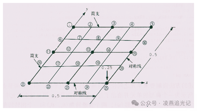
图7:边缘简支的矩形薄板
如图7所示的边缘简支的1/4对称的正方形板,划分为16个正方形单元。板受到一个集中荷载的作用,所以荷载的1/4值作用在节点25上。输入数据*.dat文件的相关内容如下:
======================================
      数值案例:矩形薄板的数据输入
======================================

x单元数nxe    y单元数nye   材料类型数np_types
   4              4              1

x单元尺寸aa   y单元尺寸bb   板厚th
   0.125       0.125        1.0

单元特征值prop(弹性模量e, 泊松比v)
  10.92    0.3

单元特性类型etype(不需要not needed)

约束节点数nr
约束节点编号k1与相应的自由度nf
16
 1 0 0 0 1       2 0 0 1 1       3 0 0 1 1   4 0 0 1 1
 5 0 0 1 0       6 0 1 0 1      10 1 0 1 0      11 0 1 0 1
15 1 0 1 0      16 0 1 0 1      20 1 0 1 0      21 0 1 0 0
22 1 1 0 0      23 1 1 0 0      24 1 1 0 0      25 1 0 0 0

受载节点数loaded_nodes
受载节点编号k2与相应的荷载loads
1
25  0.25  0.0  0.0  0.0

给定位移fixed_freedoms
0
相应的计算结果*.res如下。板中心挠度(节点25)为0.11568,很接近文献[2]精确结果0.01160。通过增加网格数量,可以得到更为精确的结果。
================================================
  数值案例:矩形薄板的各网格节点位移和单元中心弯矩
================================================

There are 64 equations and the skyline storage is 1079

  Node   Disp        Rot-x       Rot-y       Twist-xy
   1    0.0000e+00     0.0000e+00     0.0000e+00    -8.7067e-02
   2    0.0000e+00     0.0000e+00    -1.0701e-02    -8.2634e-02
   3    0.0000e+00     0.0000e+00    -2.0221e-02    -6.7652e-02
   4    0.0000e+00     0.0000e+00    -2.7049e-02    -3.9307e-02
   5    0.0000e+00     0.0000e+00    -2.9575e-02     0.0000e+00
   6    0.0000e+00     1.0701e-02     0.0000e+00    -8.2634e-02
   7    1.3166e-03     1.0187e-02    -1.0187e-02    -7.9158e-02
   8    2.4948e-03     8.4163e-03    -1.9416e-02    -6.6649e-02
   9    3.3491e-03     4.9507e-03    -2.6261e-02    -4.0251e-02
  10    3.6683e-03     0.0000e+00    -2.8873e-02     0.0000e+00
  11    0.0000e+00     2.0221e-02     0.0000e+00    -6.7652e-02
  12    2.4948e-03     1.9416e-02    -8.4163e-03    -6.6648e-02
  13    4.7674e-03     1.6500e-02    -1.6500e-02    -6.1661e-02
  14    6.4759e-03     1.0154e-02    -2.3277e-02    -4.3639e-02
  15    7.1390e-03     0.0000e+00    -2.6224e-02     0.0000e+00
  16    0.0000e+00     2.7049e-02     0.0000e+00    -3.9307e-02
  17    3.3491e-03     2.6261e-02    -4.9506e-03    -4.0251e-02
  18    6.4758e-03     2.3277e-02    -1.0154e-02    -4.3638e-02
  19    8.9874e-03     1.5874e-02    -1.5874e-02    -4.8808e-02
  20    1.0062e-02     0.0000e+00    -1.9502e-02     0.0000e+00
  21    0.0000e+00     2.9575e-02     0.0000e+00     0.0000e+00
  22    3.6683e-03     2.8873e-02     0.0000e+00     0.0000e+00
  23    7.1390e-03     2.6224e-02     0.0000e+00     0.0000e+00
  24    1.0062e-02     1.9502e-02     0.0000e+00     0.0000e+00
  25    1.1568e-02     0.0000e+00     0.0000e+00     0.0000e+00

Element  x-moment       y-moment      xy-moment
   1   -2.8285e-03    -2.8286e-03    -5.9483e-02
   2   -9.0674e-03    -7.8003e-03    -5.3279e-02
   3   -1.6090e-02    -1.0844e-02    -3.8687e-02
   4   -2.1438e-02    -1.1751e-02    -1.4474e-02
   5   -7.8001e-03    -9.0673e-03    -5.3278e-02
   6   -2.5595e-02    -2.5595e-02    -4.9588e-02
   7   -4.7688e-02    -3.6736e-02    -3.8879e-02
   8   -6.6628e-02    -4.0105e-02    -1.5735e-02
   9   -1.0844e-02    -1.6090e-02    -3.8687e-02
  10   -3.6736e-02    -4.7688e-02    -3.8879e-02
  11   -7.5262e-02    -7.5263e-02    -3.7112e-02
  12   -1.2022e-01    -8.6894e-02    -1.9747e-02
  13   -1.1751e-02    -2.1438e-02    -1.4474e-02
  14   -4.0105e-02    -6.6628e-02    -1.5735e-02
  15   -8.6893e-02    -1.2022e-01    -1.9747e-02
  16   -1.9189e-01    -1.9189e-01    -3.0319e-02
5. 结语
采用4节点板单元建立受弯薄板的二维有限元模型,能量原理推导出基尔霍夫板的刚度和弯矩的二重积分表达式,利用高斯积分法得到单元刚度矩阵和弯矩的典型表达式。组装出矩阵位移法的整体刚度矩阵,通过罚函数法处理边界条件,得到有限元方程。
采用C++语言实现算法设计。将整体刚度矩阵(稀疏矩阵)进行Cholesky分解后存储于一维向量空间,求解有限元方程,得到各单元节点的位移向量,回代得到各单元板中心的弯矩值。使用该程序计算薄板受弯问题,结果符合预期。
后续将增加图像/可视化子程序,便于调试和显示结果。
二十三,糖瓜粘;
二十四,扫房子;
二十五,冻豆腐;
二十六,去买肉;
二十七,宰公鸡;
二十八,把面发;
二十九,蒸馒头;
三十晚上熬一宿;
初一、初二满街走。
祝大家:
参考文献:
[1]: 徐秉业, 刘信声 著. 应用弹塑性力学[M]. 北京: 清华大学出版社, 1995 [2]: I. M. Smith, D. V. Griffiths, L. Margetts 著. 张新春, 慈铁军, 范伟丽 等译. 有限元方法编程(原书第五版)[M]. 北京: 电子工业出版社, 2017 [3]: T. R. Chandrupatla, A. D. Belegundu 著. 曾攀, 雷丽萍 译. 工程中的有限元法(原书第四版)[M]. 北京:机械工业出版社, 2021