几何非线性FEM 程序｜一维杆 UL格式

数值案例

考虑初始长度    、初始截面积    的两节点一维杆。节点 1 固定，节点 2 施加轴向集中力    ，尝求解节点 2 的位移    。

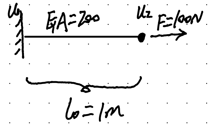
程序

import math

import numpy as np

YOUNG_MODULUS = 200.0
INITIAL_LENGTH = 1.0
INITIAL_AREA = 1.0
TARGET_FORCE = 100.0


def deformation_gradient(u):
    """Return the deformation gradient F of the uniaxial bar."""
    displacement_gradient = u / INITIAL_LENGTH

    F = np.array([
        [1.0 + displacement_gradient]
    ])

    return F


def green_lagrange_strain(F):
    """Return the Green-Lagrange strain E = 0.5 * (F.T F - I)."""
    identity = np.eye(1)

    E = 0.5 * (F.T @ F - identity)

    return E


def second_p_k_stress(E):
    """Return the second Piola-Kirchhoff stress S = Young's modulus * E."""
    S = YOUNG_MODULUS * E

    return S


def jacobian(F):
    """Return the one-dimensional Jacobian J = det(F)."""
    J = np.linalg.det(F)

    return J


def cauchy_stress(F, S, J):
    """Return the Cauchy stress sigma = (1 / J) * F S F.T."""
    sigma = (1.0 / J) * F @ S @ F.T

    return sigma


def internal_force(F, sigma, J):
    """Return the internal force obtained from the UL internal virtual work."""
    F11 = F[0, 0]
    sigma11 = sigma[0, 0]

    A = J * INITIAL_AREA / F11
    force = sigma11 * A

    return force


def tangent_stiffness(F, sigma, J):
    """Return the UL tangent stiffness Kt = k_mat + k_geo."""
    F11 = F[0, 0]
    sigma11 = sigma[0, 0]

    A = J * INITIAL_AREA / F11
    L = F11 * INITIAL_LENGTH

    k_mat = YOUNG_MODULUS * A * F11 ** 3 / L
    k_geo = sigma11 * A / L

    tangent = k_mat + k_geo

    return tangent


def calculate_state(u):
    """Calculate all physical quantities from the current displacement."""
    F = deformation_gradient(u)
    E = green_lagrange_strain(F)
    S = second_p_k_stress(E)

    J = jacobian(F)
    sigma = cauchy_stress(F, S, J)
    force = internal_force(F, sigma, J)

    return F, E, sigma, J, force


def convergence_residual(residual, target_force):
    """Return the normalized squared residual used in the original example."""
    return residual**2 / (1.0 + target_force**2)


def newton_raphson(
    initial_u,
    target_force,
    tol=1.0e-5,
    max_iter=20,
):
    """Solve one load increment with the Newton-Raphson method."""
    trial_u = float(initial_u)
    iteration = 0

    F, E, sigma, J, force = calculate_state(trial_u)
    residual = target_force - force
    conv_residual = convergence_residual(residual, target_force)

    print(
        f"{'iter':>5} {'u2':>10} {'E11':>10} "
        f"{'sigma11':>12} {'conv_R':>12}"
    )
    print(
        f"{iteration:5d} {trial_u:10.5f} {E[0, 0]:10.5f} "
        f"{sigma[0, 0]:12.3e} {conv_residual:12.3e}"
    )

    while conv_residual > tol and iteration < max_iter:
        tangent = tangent_stiffness(F, sigma, J)
        if math.isclose(tangent, 0.0, abs_tol=1.0e-14):
            raise ZeroDivisionError("Zero tangent stiffness.")

        delta_u = residual / tangent
        trial_u += delta_u

        iteration += 1
        F, E, sigma, J, force = calculate_state(trial_u)
        residual = target_force - force
        conv_residual = convergence_residual(residual, target_force)

        print(
            f"{iteration:5d} {trial_u:10.5f} {E[0, 0]:10.5f} "
            f"{sigma[0, 0]:12.3e} {conv_residual:12.3e}"
        )

    converged = conv_residual <= tol

    return trial_u, iteration, converged

结果汇总

固定步长

自动步长

结果分析

从上面数据还有之前的 TL 格式的数据，可以看到两个现象：

1. UL 格式下的应力收敛于 100N，这与施加的外力是一致的，而 TL 的应力小于该值
2. UL 格式下的应变小于 TL 格式下的应变

UL 输出的是当前构形下的 Cauchy 应力    ，内力为    ；当前算例中面积    ，因此 Cauchy 应力的数值恰好等于外力100，但严格来说应力与力的单位并不相同。

TL 输出的是第二 P–K 应力    ，其内力为    ，拉伸时，所以达到相同的100外力时，    必然小于100。

应变也是同样的道理：TL 的 Green–Lagrange 应变相对于初始长度描述变形，而 UL 输出的空间应变相对于拉伸后的当前长度描述变形；由于当前长度大于初始长度，相同伸长量除以当前长度所得的空间应变自然更小。

因此，应力和应变数值的差异只是构形和度量方式不同，两种格式描述的是同一个变形与平衡状态。