计算流体动力学核心方法与求解技术

计算流体动力学核心方法与求解技术(Computational Methods for Fluid Dynamics)
摘要:
本文为 Ferziger 与 Peric 所著《计算流体动力学数值方法》第三版,系统讲解 CFD 数值求解全套理论。全书从流体守恒控制方程切入,依次介绍有限差分、有限体积两类主流离散方法,推导一 / 二阶导数、各类插值格式;阐述高斯消元、TDMA、多重网格、共轭梯度等线性方程组求解算法,包含松弛、延迟修正、牛顿线性化等非线性处理手段。书中兼顾结构化 / 非结构化网格、动网格、湍流模拟、可压缩流等工程场景,配套一维对流扩散等验证算例,分析截断误差、迭代误差与收敛判定方法,兼顾理论推导与程序实现思路,是 CFD 离散算法与求解器开发经典教材。
Preface
Computational fluid dynamics,commonly known by the acronym 'CFD’, is undergoing significant expansion in terms of both the number of courses offered at universities and the number of researchers active in the field.There are a number of software packages available that solve fluid flow problems;the market is not quite as large as the one for structural mechanics codes,in which finite element methods are well established.The lag can be explained by the fact that CFD problems are,in general,more difficult to solve.However,CFD codes are slowly being accepted as design tools by industrial users.At present, users of CFD need to be fairly knowledgeable,which requires education of both students and working engineers.The present book is an attempt to fill this need.
It is our belief that,to work in CFD,one needs a solid background in both fluid mechanics and numerical an alysis;significant errors have been made by people lacking knowledge in one or the other.We therefore encourage the reader to obtain a working knowledge of these subjects before entering into a study of the material in this book.Because different people view numeri- cal methods differently,and to make this work more self-contained,we have included two chapters on basic numerical methods in this book.The book is based on material offered by the authors in courses at Stanford Univer- sity,the University of Erlangen-Nürnberg and the Technical University of Hamburg-Harburg.It reflects the authors'experience in both writing CFD codes and using them to solve engineering problems.Many of the codes used in the examples,from the simple ones involving rectangular grids to the ones using non-orthogonal grids and multigrid methods,are available to interested readers;see the information on how to access them via Internet in the ap- pendix.These codes illustrate the methods described in the book;they can be adapted to the solution of many fluid mechanical problems.Students should try to modify them(e.g.to implement different boundary conditions,interpo- lation schemes,differentiation and integration approximations,etc.).This is important as one does not really know a method until s/he has programmed and/or run it.
Since one of the authors(M.P.)has just recently decided to give up his pro- fessor position to work for a provider of CFD tools,we have also included in the Internet site a special version of a full-featured commercial CFD package that can be used to solve many different flow problems.This is accompanied by a collection of prepared and solved test cases that are suitable to learn how to use such tools most effectively.Experience with this tool will be valu- able to anyone who has never used such tools before,as the major issues are common to most of them.Suggestions are also given for parameter variation, error estimation,grid quality assessment,and efficiency improvement.
The finite volume method is favored in this book,although finite difference methods are described in what we hope is sufficient detail.Finite element methods are not covered in detail as a number of books on that subject already exist.
We have tried to describe the basic ideas of each topic in such a way that they can be understood by the reader;where possible,we have avoided lengthy mathematical ana lysis.Usually a general description of an idea or method is followed by a more detailed description (including the necessary equations)of one or two numerical schemes representative of the better meth- ods of the type;other possible approaches and extensions are briefly de- scribed.We have tried to emphasize common elements of methods rather than their differences.
There is a vast literature devoted to numerical methods for fluid mechan- ics.Even if we restrict our attention to incompressible flows,it would be impossible to cover everything in a single work.Doing so would create con- fusion for the reader.We have therefore covered only the methods that we have found valuable and that are commonly used in industry in this book. References to other methods are given,however.
We have placed considerable emphasis on the need to estimate numerical errors;almost all examples in this book are accompanied with error ana lysis. Although it is possible for a qualitatively incorrect solution of a problem to look reasonable (it may even be a good solution of another problem),the consequences of accepting it may be severe.On the other hand,sometimes a relatively poor solution can be of value if treated with care.Industrial users of commercial codes need to learn to judge the quality of the results before believing them;we hope that this book will contribute to the awareness that numerical solutions are always approximate.
We have tried to cover a cross-section of modern approaches,including di- rect and large eddy simulation of turbulence,multigrid methods and parallel computing,methods for moving grids and free surface flows,etc.Obviously, we could not cover all these topics in detail,but we hope that the informa- tion contained herein will provide the reader with a general knowledge of the subject;those interested in a more detailed study of a particular topic will find recommendations for further reading.
While we have invested every effort to avoid typing,spelling and other errors,no doubt some remain to be found by readers.We will appreciate your notifying us of any mistakes you might find,as well as your comments and suggestions for improvement of future editions of the book.For that purpose,the authors'electronic mail addresses are given below.We also hope that colleagues whose work has not been referenced will forgive us,since any omissions are unintentional.
We have to thank all our present and former students,colleagues,and friends,who helped us in one way or another to finish this work;the complete list of names is too long to list here.Names that we cannot avoid mentioning include Drs.Ismet Demirdžic,Samir Muzaferija,Željko Lilek,Joseph Oliger, Gene Golub,Eberhard Schreck,Volker Seidl,Kishan Shah,Fotina(Tina) Katapodes and David Briggs.The help provided by those people who created and made available TEX,ITEX,Linux,Xfig,Ghostscript and other tools which made our job easier is also greatly appreciated.
Our families gave us a tremendous support during this endeavor;our special thanks go to Anna,Robinson and Kerstin Peric and Eva Ferziger.
This collaboration between two geographically distant colleagues was made possible by grants and fellowships from the Alexander von Humboldt Foundation and the Deutsche Forschungsgemeinschaft(German National Re- search Organization).Without their support,this work would never have come into existence and we cannot express sufficient thanks to them.
Milovan Peric
milovan@cd.co.uk Joel H.Ferziger
ferziger@leland.stanford.edu
1.Basic Concepts of Fluid Flow
1.1 Introduction
Fluids are substances whose molecular structure offers no resistance to exter- nal shear forces:even the smallest force causes deformation of a fuid particle. Although a significant distinction exists between liquids and gases,both types of fuids obey the same laws of motion.In most cases of interest,a fluid can be regarded as continuum,i.e.a continuous substance.
Fluid flow is caused by the action of externally applied forces.Common driving forces include pressure differences,gravity,shear,rotation,and sur- face tension.They can be classified as surface forces (e.g. the shear force due to wind blowing above the ocean or pressure and shear forces created by a movement of a rigid wall relative to the fluid)and body forces(e.g.gravity and forces induced by rotation).
While all fuids behave similarly under action of forces,their macroscopic properties differ considerably.These properties must be known if one is to study fuid motion;the most important properties of simple fluids are the density and viscosity.Others,such as Prandtl number,specific heat,and sur- face tension affect fuid flows only under certain conditions,e.g.when there are large temperature differences.Fluid properties are functions of other ther- modynamic variables (e.g.temperature and pressure);although it is possible to estimate some of them from statistical mechanics or kinetic theory,they are usually obtained by laboratory measurement.
Fluid mechanics is a very broad field.A small library of books would be required to cover all of the topics that could be included in it.In this book we shall be interested mainly in flows of interest to mechanical engineers but even that is a very broad area so we shall try to classify the types of problems that may be encountered.A more mathematical,but less complete,version of this scheme will be found in Sect.1.8.
The speed of a flow affects its properties in a number of ways.At low enough speeds,the inertia of the fuid may be ignored and we have creep- ing flow.This regime is of importance in flows containing small particles (suspensions),in flows through porous media or in narrow passages (coating techniques,micro-devices).As the speed is increased,inertia becomes im- portant but each fluid particle follows a smooth trajectory;the flow is then said to be laminar.Further increases in speed may lead to instability that eventually produces a more random type of flow that is called turbulent;the process of laminar-turbulent transition is an important area in its own right. Finally,the ratio of the flow speed to the speed of sound in the fluid(the Mach number)determines whether exchange between kinetic energy of the motion and internal degrees of freedom needs to be considered.For small Mach numbers,Ma<0.3,the flow may be considered incompressible;other- wise,it is compressible.If Ma<1,the flow is called subsonic;when Ma>1, the flow is supersonic and shock waves are possible.Finally,for Ma>5,the compression may create high enough temperatures to change the chemical nature of the fuid;such flows are called hypersonic.These distinctions affect the mathematical nature of the problem and therefore the solution method. Note that we call the flow compressible or incompressible depending on the Mach number,even though compressibility is a property of the fluid.This is common terminology since the flow of a compressible fuid at low Mach number is essentially incompressible.
In many flows,the effects of viscosity are important only near walls,so that the flow in the largest part of the domain can be considered as inviscid. In the fuids we treat in this book,Newton's law of viscosity is a good ap- proximation and it will be used exclusively.Fluids obeying Newton's law are called Newtonian;non-Newtonian fluids are important for some engineering applications but are not treated here.
Many other phenomena affect fluid flow.These include temperature dif- ferences which lead to heat transfer and density differences which give rise to buoyancy. They,and differences in concentration of solutes,may affect flows significantly or,even be the sole cause of the flow.Phase changes(boiling, condensation,melting and freezing),when they occur,always lead to impor- tant modifications of the flow and give rise to multi-phase flow.Variation of other properties such as viscosity,surface tension etc.may also play impor- tant role in determining the nature of the flow.With only a few exceptions, these effects will not be considered in this book.
In this chapter the basic equations governing fuid flow and associated phenomena will be presented in several forms:(i)a coordinate-free form, which can be specialized to various coordinate systems,(ii)an integral form for a finite control volume,which serves as starting point for an important class of numerical methods,and(iii)a differential(tensor)form in a Cartesian reference frame,which is the basis for another important approach.The basic conservation principles and laws used to derive these equations will only be briefly summarized here;more detailed derivations can be found in a number of standard texts on fluid mechanics (e.g.Bird et al.,1962;Slattery, 1972;White,1986).It is assumed that the reader is somewhat familiar with the physics of fluid flow and related phenomena,so we shall concentrate on techniques for the numerical solution of the governing equations.
1.2 Conservation Principles
Conservation laws can be derived by considering a given quantity of matter or control mass(CM)and its ertensive properties,such as mass,momentum and energy.This approach is used to study the dynamics of solid bodies,where the CM (sometimes called the system)is easily identified.In fuid flows,however, it is difficult to follow a parcel of matter.It is more convenient to deal with the flow within a certain spatial region we call a control volume(CV),rather than in a parcel of matter which quickly passes through the region of interest. This method of ana lysis is called the control volume approach
We shall be concerned primarily with two extensive properties,mass and momentum.The conservation equations for these and other properties have common terms which will be considered first.
The conservation law for an extensive property relates the rate of change of the amount of that property in a given control mass to externally deter- mined effects.For mass,which is neither created nor destroyed in the flows of engineering interest,the conservation equation can be written:
 (1.1)
(1.1)
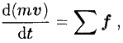
On the other hand,momentum can be changed by the action of forces and its conservation equation is Newton's second law of motion:
 (1.2)
(1.2)
where t stands for time,m for mass,v for the velocity,and f for forces acting on the control mass.
We shall transform these laws into a control volume form that will be used throughout this book.The fundamental variables will be intensive rather than extensive properties;the former are properties which are independent of the amount of matter considered.Examples are density p(mass per unit volume) and velocity v (momentum per unit mass).
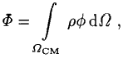
Ifφ is any conserved intensive property(for mass conservation,φ=1;for momentum conservation,φ=v;for conservation of a scalar,φrepresents the conserved property per unit mass),then the corresponding extensive property Φcan be expressed as:
 (1.3)
(1.3)
where ΩcM stands for volume occupied by the CM.Using this definition, the left hand side of each conservation equation for a control volume can be written·1
¹This equation is often called control volume equation or the Reynolds'transport
 (1.4)
(1.4)
where Ωcv is the CV volume,Scv is the surface enclosing CV,n is the unit vector orthogonal to Scv and directed outwards,v is the fluid velocity and vb is the velocity with which the CV surface is moving.For a fixed CV,which we shall be considering most of the time,Ub=0 and the first derivative on the right hand side becomes a local(partial)derivative.This equation states that the rate of change of the amount of the property in the control mass,Φ,is the rate of change of the property within the control volume plus the net flux of it through the CV boundary due to fluid motion relative to CV boundary.The last term is usually called the convective(or sometimes, advective)flux of φ through the CV boundary.If the CV moves so that its boundary coincides with the boundary of a control mass,then u=Ub and this term will be zero as required.
A detailed derivation of this equation is given in in many textbooks on fluid dynamics(e.g.in Bird et al.,1962;Fox and McDonald,1982)and will not be repeated here.The mass,momentum and scalar conservation equations will be presented in the next three sections.For convenience,a fixed CV will be considered;Ω represents the CV volume and S its surface.
1.3 Mass Conservation
The integral form of the mass conservation (continuity)equation follows di- rectly from the control volume equation,by settingφ=1:
 (1.5)
(1.5)
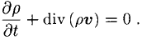
By applying the Gauss'divergence theorem to the convection term,we can transform the surface integral into a volume integral.Allowing the control volume to become infinitesimally small leads to a differential coordinate-free form of the continuity equation:
 (1.6)
(1.6)
This form can be transformed into a form specific to a given coordinate system by providing the expression for the divergence operator in that system. Expressions for common coordinate systems such as the Cartesian,cylindrical and spherical systems can be found in many textbooks(e.g.Bird et al.,1962); expressions applicable to general non-orthogonal coordinate systems are given e.g.in Truesdell(1977),Aris(1989),Sedov(1971).We present below the Cartesian form in both tensor and expanded notation.Here and throughout this book we shall adopt the Einstein convention that whenever the same
index appears twice in any term,summation over the range of that index is implied:
 (1.7)
(1.7)
where xi(i=1,2,3)or(x,y,z)are the Cartesian coordinates and ui or (ux,uy,uz)are the Cartesian components of the velocity vector v.The con- servation equations in Cartesian form are often used and this will be the case in this work.Differential conservation equations in non-orthogonal coordi- nates will be presented in Chap.8.
原资料见附件
免责声明:
本页面/内容部分素材来源于互联网公 开 信 息,旨在传递更多信息,不代表本平台立场。
版权归原作者或机构所有,如涉及侵权,请通过平台联系我们,我们将在核实后第一时间处理。
本平台对转载内容的真实性、准确性不作任何保证,用户需自行判断并承担使用风险。