AQWA-WAVE 用户手册(aqwa-wave)

摘要:
本文为 ANSYS AQWA-WAVE Version 12 官方用户手册,聚焦波浪载荷向有限元模型传递的核心功能。手册系统阐述水动力绕射 / 辐射力、莫里森方程惯性与拖曳力、流耦合的理论基础,详细说明输入文件格式、结构与水动力模型对接、工况定义、坐标系转换、单位换算及载荷映射流程。支持管单元、梁单元、壳 / 实体单元载荷分配,提供固定 / 浮式结构、对称模型、环形与杆件载荷赋值方法,兼容中性文件接口,可对接 ASAS 与 ANSYS。文档含命令说明、算例与旧版格式对照,为海洋平台、船舶等结构的波浪载荷施加提供完整操作指南。
AQWA-WAVE User Manual
Hydrodynamic Load Transfer
Version 12 April 2009
Century Dynamics Limited Suite 1, 3 Horsham Gates
North Street Horsham
West Sussex RH13 5PJ
ENGLAND
Telephone +44 (0) 1403 270066 Fax +44 (0) 1403 270099
Email support-uk@ansys.com
URL www.ansys.com/customerportal
Copyright 2009. Century Dynamics Limited. All Rights Reserved.
Century Dynamics is a subsidiary ofANSYS, Inc.
Unauthorised use, distribution or duplication is prohibited
Revision Information
The information in this guide applies to all ANSYS, Inc. products released on or after this date, until superseded by a newer version of this guide. This guide replaces individual product installation guides from previous releases.
Copyright and Trademark Information
ANSYS, ANSYS Workbench, CFX, AUTODYN, ASAS, AQWA and any and all ANSYS, Inc. product and service names are registered trademarks or trademarks ofANSYS, Inc. or its subsidiaries located in the United States or other countries. ICEM CFD is a trademark licensed by ANSYS, Inc.
ABAQUS is a registered trademark of ABAQUS, Inc
Adobe and Acrobat are registered trademarks of Adobe Systems Incorporated Compaq is a registered trademark of Compaq Computer Corporation
Delphi is a registered trademark of Borland Software Corporation
DXF is a trademark of Autodesk, Inc
FEMGV, FEMGEN and FEMVIEW are trademarks ofFemsys Limited
FLEXlm and FLEXnet are registered trademarks of Macrovision Corporation Formula One is a trademark of Visual Components, Inc
GINO is a registered trademark of Bradly Associates Ltd IGES is a trademark ofIGES Data An alysis, Inc
Intel is a registered trademark of Intel Corporation
Mathcad is a registered trademark of Mathsoft Engineering & Education, Inc.
Microsoft, Windows, Windows 2000, Windows XP and Excel are registered trademarks of Microsoft Corporation NASTRAN is a registered trademark of the National Aeronautics and Space Administration.
PATRAN is a registered trademark of MSC Software Corporation SentinelSuperPro™ is a trademark of Rainbow Technologies, Inc SESAM is a registered trademark of DNV Software
Softlok is a trademark of Softlok International Ltd
All other trademarks or registered trademarks are the property of their respective owners.
Disclaimer Notice
THIS ANSYS SOFTWARE PRODUCT AND PROGRAM DOCUMENTATION INCLUDE TRADE SECRETS AND ARE CONFIDENTIAL AND PROPRIETARY PRODUCTS OF ANSYS, INC., ITS SUBSIDIARIES, OR LICENSORS. The software products and documentation are furnished by ANSYS, Inc., its subsidiaries, or affiliates under a software license agreement that contains provisions concerning non-disclosure, copying, length and nature of use, compliance with exporting laws, warranties, disclaimers, limitations of liability, and remedies, and other provisions. The software products and documentation may be used, disclosed, transferred, or copied only in accordance with the terms and conditions of that software license agreement.
ANSYS, Inc. and ANSYS Europe, Ltd. are UL registered ISO 9001:2000 Companies.
U.S. Government Rights
For U.S. Government users, except as specifically granted by the ANSYS, Inc. software license agreement, the use, duplication, or disclosure by the United States Government is subject to restrictions stated in the ANSYS, Inc. software license agreement and FAR 12.212 (for non-DOD licenses).
Third-Party Software
The products described in this document contain the following licensed software that requires reproduction of the following notices.
Copyright 1984-1989, 1994 Adobe Systems Incorporated. Copyright 1988, 1994 Digital Equipment Corporation.
Permission to use, copy, modify, distribute and sell this software and its documentation for any purpose and without fee is hereby granted, provided that the above copyright notices appear in all copies and that both those copyright notices and this permission notice appear in supporting documentation, and that the names of Adobe Systems and Digital Equipment Corporation not be used in advertising or publicity pertaining to distribution of the software without specific, written prior permission. Adobe Systems & Digital Equipment Corporation make no representations about the suitability of this software for any purpose. It is provided "as is" without express or implied warranty.
Advanced Visual Systems
All rights reserved. Use of this software is subject to the terms of the agreement with Advanced Visual Systems Inc. or its distributors and licensee. Use, duplication or disclosure by the Federal Government is subject to the restrictions set forth in FAR 52.227-19(c), Commercial Computer Software or, for Department of Defense users, by DFAR
252.227-7202.3.
Formula One is a trademark of Visual Components, Inc.
The product contains Formula One from Visual Components, Inc. Copyright 1994- 1995. All rights reserved. Microsoft, Windows, Windows 2000 and Windows XP are registered trademarks of Microsoft Corporation whirlgif
Copyright (c) 1997, 1998, 1999 by Hans Dinsen-Hansen Copyright (c) 1995, 1996 by Kevin Kadow
Copyright (c) 1990, 1991, 1992 by Mark Podlipec.
All rights reserved. This software may be freely copied, modified and redistributed
without fee provided that this copyright notice is preserved intact on all copies and modified copies.
There is no warranty or other guarantee of fitness of this software.
It is provided solely "as is". The author(s) disclaim(s) all responsibility and liability with respect to this software's usage or its effect upon hardware or computer systems.
The Graphics Interchange format (c) is the Copyright property ofCompuserve Incorporated. Gif(s m) is a Service Mark property ofCompuserve Incorporated.
The ANSYS third-party software information is also available via download from the Customer Portal on the ANSYS
web page. If you are unable to access the third-party legal notices, please contact ANSYS, Inc.
Published in the United Kingdom
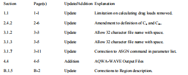
AQWAWAVE User Manual Update Sheet for Version 12
AQWAWAVE User Manual Version 12
10 February 2009
Modifications:
The following modifications have been incorporated:
1. INTRODUCTION
1.1 Overview
AQWA-WAVE forms part of the ASAS™ and AQWA™ suites of programs developed by Century Dynamics Limited. Its function is to transfer wave loads on fixed or floating structures (calculated by the radiation/diffraction program, AQWA-LINE) to a finite element, structural an alysis package.
AQWA-WAVE forms a link between the AQWA and ASAS suites of programs. It can also output wave loads to the ANSYS® system. AQWA-WAVE also has the ability to read in structural and hydrodynamic data defined in neutral format and output the wave loads in neutral format. This facility permits the program to interface with a range of hydrodynamic and FE programs.
AQWA-LINE uses a mesh composed of panels, or facets, to model the structure. It calculates pressures at the facet centroids, due to the incident, diffracted and radiated waves, for a range of wave periods and directions specified by the user.
The pressures calculated by AQWA-LINE effectively relate to waves of unit amplitude. These pressures therefore have to be scaled by AQWA-WAVE to relate to the actual wave height required by the AQWA- WAVE user.
AQWA-WAVE can be used to transfer facet loads to one of two types of structural model:
• a simplified, normally single component, stick model, in which only tube or beam elements are subject to hydrodynamic loads
• a single or multi-component model, in which hydrodynamic loads act mainly upon the wetted surfaces of shell or brick elements.
In the case of brick elements, a special load case is required in the ASAS master component file, to identify which faces ofthe brick are wetted.
As AQWA-LINE uses linear wave theory, it cannot calculate drag forces. Provision is therefore made for AQWA-WAVE to calculate the drag forces, including the effect of current. The program also allows for both drag and inertial forces to be calculated for additional structural elements in the FE model, which are too s mall to be modelled using AQWA-LINE facets.
AQWA-WAVE evaluates all forces at a particular phase in the wave cycle. The user can request many wave cases (specified by wave period, wave direction, wave height, wave phase and current profile) in a single run of the program.
When AQWA-WAVE is executed, the program reads a complete set ofFE input data files and writes out a new set with all the necessary load cases inserted. For floating structures, balancing accelerations are also written into the output FE files.
There are currently a number of program limitations, which should be noted by the user:
• AQWA-WAVE does not currently recognise either OFFSETS or LOCAL AXES defined for tube or beam elements in the ASAS geometry (GEOM) deck. The user must not therefore define such items in this deck.
• When setting up an ASAS model using SHELL type elements, the user must ensure that the input order of the nodes is anti-clockwise, when viewing the wetted surface of the element (the same convention as in AQWA-LINE).
1.2 Manual Layout
Section2discusses the theoretical basis of the AQWA-WAVE program.
Section3gives a detailed explanation of the AQWA-WAVE data format from Version 14.03. Section4gives information on how to run the program.
Section5provides an example of program use.
AppendixAgives a detailed explanation of the AQWA-WAVE data format up to Version 14.02. Appendix Bgives a detailed explanation of the AQWA-WAVE neutral file formats.
2. THEORY
2.1 Program Structures
AQWA-WAVE is currently run as a post-processor to AQWA-LINE to transfer the facet pressures from AQWA™ to a structural model created using ASAS™ data. Optionally, drag and inertia loads on tubular components of the structure may be calculated and added to the diffraction/radiation forces from AQWA-LINE.
The ASAS model may comprise 1D or 3D elements. Typical 1D elements are tubes and beams. The elements that may be loaded by AQWA-WAVE are:
TUBE BEAM BM3D
Groups ofAQWA facets may be associated with each tube or node in the ASAS model and diffraction/radiation forces assigned accordingly. (The user should decide how the facet loads are to be distributed, before running AQWA-LINE, so that appropriate element groupings can be set up in that run.) Drag and inertia loads on the tubes can also be calculated and added to these forces using Morison’s equation.
3D structures comprise solid or shell elements. The elements that may be loaded by AQWA-WAVE are:

Diffraction radiation forces are once again transferred to these elements, this time by interpolation of facet pressures to the wetted external surface of the elements. Drag forces on the same surfaces can be calculated by the program and again assigned as pressures to the elements.
The ASAS model may be subdivided into components. AQWA-WAVE can load these components according to their position in the final assembled model. Load assembly data will be produced that will allow the ASAS runs to proceed with no further data editing.
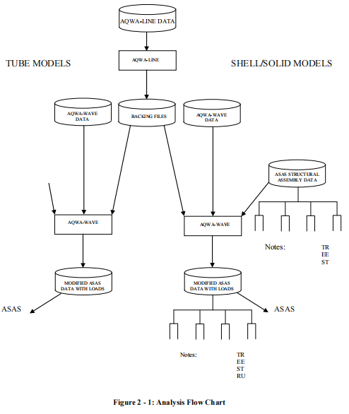
Figure 2 - 1shows the data flow and program structure for a typical ana lysis using AQWA-LINE and AQWA- WAVE. As can be seen, the AQWA-LINE run is completed first and backing files stored. These same backing files may be used for both 1D and 3D model runs, the type of run being defined in the AQWA-WAVE data file. This file also defines the load cases required from the AQWA-LINE run and the file name for the ASAS model. In the figure, the possibility that the 3D model may be a component an alysis is shown. In this event, the program will automatically search for component data files, applying loads and rewriting the data as required.
AQWA-WAVE can also transfer AQWA facet pressures to ANSYS® . In order to use this facility, the user must first create an equivalent ASAS model from the ANSYS model using the ANSTOASAS macro in ANSYS. After running AQWA-WAVE, the structural loading generated can be imported back to the ANSYS model using the /INPUT command while in the solution processor. The interface to ANSYS currently has the following limitations:
• Hydrodynamic loads on beams are ignored (loads on PIPE type elements can be transferred, however).
• The structural model must be modelled as a single structure, i.e. no sub-structure components.
2.2 Selection of Wave Cases
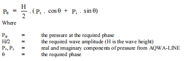
A large number of wave cases may be selected by the user in the AQWA-WAVE data. This is achieved by defining a wave frequency number and a wave direction number from the preceding AQWA-LINE data and then specifying a wave height and phase to be associated with them. The wave height is required since the AQWA-LINE run is for unit wave amplitude and must be scaled to the required height. The phase is necessary as the drag forces that can be produced by the program generally do not vary sinusoidally and cannot be represented dynamically as in AQWA-LINE.
Pressures from the AQWA-LINE an alysis are then extracted from the backing files and evaluated for the selected height/phase as follows:
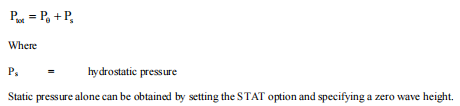
Optionally, static pressures may be calculated and added to the above time varying pressures by the setting of the ‘STAT’ option in the AQWA-WAVE data. The revised pressure is then simply given as:
Load cases created by AQWA-WAVE will be written before any other ASAS load cases and will be sequenced from 1001 unless the user specifies a different load case offset (See LCOF command in Section3.1.5).
2.3 Incident Diffracted and Radiated Wave Forces
Incident, diffracted and radiated wave forces on the structure are calculated by AQWA-LINE for selected wave periods and directions. These forces may be thought of as relating to a unit wave amplitude, although they are actually forces per unit wave amplitude and relate to infinitesimal waves. The incident wave forces are sometimes referred to as Froude-Krylov forces. The radiated wave forces are zero for a fixed structure. AQWA-LINE stores the incident, diffracted and radiated components of the pressures on the individual facets in a backing file. Real and imaginary components of pressure are retained. The way AQWA-WAVE handles these pressures depends on the type of ASAS model being loaded, tube/beam models or shell/solid models.
For tube/beam models, groups ofAQWA facets (specified by element group numbers) may be associated with a given node or element in the ASAS model. This data is provided in the AQWA-WAVE data file. In addition to the group number, the user must also specify which quadrant or half of a symmetric model is to be used. Provision is also made for defining the assembled component to which the element or node belongs.
The program will evaluate the incident and diffracted wave forces for each facet in the AQWA group at the requested wave height, period, direction and phase (see Section 2.2). It will then sum these forces about the node or element centroid requested. Summed forces at a node will be applied as ASAS Nodal Loads. Forces on an element will be applied as distributed loads. Elements and nodes that do not have AQWA groups assigned to them will not be loaded.
For solid/shell elements, a special load case (load case 1000) must be present in the ASAS data for any component that has an external wetted surface. Components with no load case 1000 will be assumed to be wholly internal, or above the water surface. This load case should be an ASAS face pressure or unit load case, defining the wetted faces of all wetted elements. (Note: The actual load values are unimportant, only the face data is used by AQWA-WAVE.)
AQWA-WAVE evaluates pressures for the requested wave height, period, direction and phase, in accordance with Section2.2, for each node on the wetted surface of each element that appears in load case 1000. Elements in the ASAS model generally will not correspond to facets in the AQWA model and some method is clearly needed to obtain these pressures at the ASAS nodes. The method currently adopted is to locate the ASAS node on the AQWA mesh and then interpolate the pressure.
2.4 Morison Loads
AQWA-LINE does not evaluate drag forces on submerged components. AQWA-WAVE therefore allows Morison forces on such components to be calculated and added to the incident and diffracted wave forces from AQWA-LINE.
Two types of component are considered here:
1. Relatively large diameter tubular components simulated using facets in AQWA-LINE, but for which drag loads are considered important (e.g. GBS shafts)
2. S maller diameter tubular members subject to drag and inertia loads (e.g. conductor framing on GBS). Although provision is made for modelling the inertia loads on such tubes in AQWA-LINE, this is not the recommended modelling for AQWA-WAVE, and the tubular members do not need to be modelled in AQWA-LINE.
When evaluating Morison loads on such components of the structure, several factors need to be considered:
• The incident flow is expected to be modified by the presence of the main structure due to diffracted wave forces. The particle velocities and accelerations on which the Morison forces are based need to consider this effect.
• The local water surface during the passage of a wave is also expected to be modified due to the presence of the structure, thus affecting the extent of structure subjected to wave loading. A ‘caisson effect’ (overall increase in water height) and a ‘ride up’ on vertical members cutting the surface are expected.
• The effects of current velocity on drag should be considered. Current velocities should also be modified to allow for the presence of the structure.
• Although linear wave theory is considered sufficient for evaluating incident and diffracted wave effects, this is often not sufficient for drag loads near the water surface where the particle velocities and water surface elevation can often be in excess of that predicted by simple Airy theory. Some consideration should be given to the effects of higher order wave theory.
• The method of modelling of the ASAS structure should be considered. Although the application of drag and inertia loads to tube elements is relatively straightforward, some further rule needs to be provided to assign pressures to tubular structures defined by plate or solid elements.
The above considerations are addressed in the following two sections under the headings of fluid flow and load application.
2.4.1 Fluid Flow
At any point in the flow outside the AQWA facet model, the incident and diffracted wave flow potential can be calculated using the same Green’s function routines as AQWA-LINE. The rate of change of potential in each principal direction gives the velocity of the flow for that direction. The effect of all contributing facets is considered. These can be added as a vector to the incident flow to give the disturbed flow around the structure. Water particle accelerations are derived simply from the rate of change of velocity.
A current profile (variation of current with depth) may be specified in the AQWA-WAVE data for each wave case and phase selected from the AQWA-LINE ana lysis. The current flow is assumed to be horizontal but the direction may vary with depth. For each given point, a current velocity is then calculated by linear interpolation to the required depth. This velocity is again summed as a vector to the wave velocity in the disturbed flow, calculated as above. The user-defined current profile is assumed to include the effects of the structure disturbing the flow. The program does not modify the current velocities as it does for waves. Principles of momentum preservation or even runs of AQWA-LINE with the current represented as a long duration wave may be helpful in determining this modified profile.
Flow around a massive object tends to cause a local distortion of the still water surface known as a ‘caisson effect’ and water tends to ‘ride up’ members that cut the water surface. The latter effect is normally not considered to significantly change global load on the structure, but is of some importance to local design, particularly wave slam, slap and the determination of the required air gap. The ‘caisson effect’ is significant on GBS type structures and can result in the total load being applied higher up in the structure. AQWA-WAVE calculates most of this effect, which is due to the diffracted wave. (The increase in wave elevation due to diffraction may be obtained explicitly, using the field point facility in AQWA-LINE. The pressure at a given point at the still water level may be obtained using this method and the dynamic displacement of the water surface may be derived from the simple h = p/(ρg) formulation.)
The effect of this artificial raising of the water surface is simply to increase (or decrease if negative) the extent of structure subject to water pressure loads. If a positive value is found, the undisturbed water-surface motions are assumed to apply over the increase in depth. Otherwise, the motions are cut off at the reduced water surface.
Higher order wave theory may produce higher loads than simple Airy theory and typically account for a raising of the water surface elevation at the crest and a s moothing of the trough. Although not dealt with explicitly by AQWA-WAVE, the user can attempt to model the effect by inputting a scaled-up wave height, obtained using a suitable scaling factor. It is suggested that an estimate for this factor be obtained from a program that does allow for different wave theories, such as ASAS-WAVE.
2.4.2 Load Application
S mall diameter tubular members are handled as below:
• The water surface elevations at the ends of the element are evaluated with due allowance for the local increase or decrease mentioned above.
• If both ends of the element are below the water surface, then the member is fully loaded.
• If neither end of the element is below the water surface, then the member is unloaded.
• If only one end of the element is in the water, the member is loaded over the wetted length only.
• The fluid flow at each end of a loaded length is evaluated in accordance with2.4.1.
• The fluid flows at each loaded end are transformed into loads per unit length perpendicular to the member using Morison’s equation as below:
F = 0.5ρCd Du u + Cm ρAa
Where
F = the force per unit length
Cd = the drag coefficient
ρ = the mass density of water
D = the member diameter
u = the instantaneous velocity resolved normal to the member
Cm = the inertia coefficient
A = the cross-sectional area = πD2/4
a = instantaneous acceleration resolved normal to the member
Note: Cm = 1 + Ca
Where
Ca = the added mass coefficient.
The added mass can be ignored by setting Cm to zero. However, if Cm is set to a value less than one, but not zero, a negative Ca will be used as the Cm = 1 + Ca relationship is respected, hence the valid values for Cm are 0 or ≥1.
The user should take into account marine growth when inputting the diameter into the AQWA-WAVE data.
The drag and inertia coefficients can be defined explicitly by the user for all tube elements in the ASAS model. Members with no coefficients will not be considered. The coefficients occur in the AQWA- WAVE data and are referenced by ASAS element number and assembled component name.
• Distributed loads on the element are written to the output data file as ASAS ‘BL6' type distributed loads.
Note: The user must not define either OFFSETS or LOCAL AXES for tube elements in the ASAS geometry deck.
Large AQWA substructures, which have cylindrical symmetry (such as the shaft of a GBS) and which have been modelled in AQWA-LINE using PLATE elements can also have their drag loads calculated by AQWA- WAVE. Such substructures are referred to here as ‘AQWA components’. (An AQWA component will correspond to one or more ASAS components.)
Ignoring current for the moment, the flow ‘seen by’ an AQWA component, at any instant of time, is taken to be the flow which, at that instant, is being exactly cancelled (normal to every plate) by the combined flow due to all the hydrodynamic sources on the component. The flow ‘seen by’ the component can thus be calculated by adding, to the incident flow (assumed undisturbed), the flow due to all the hydrodynamic sources on the whole AQWA structure, EXCEPT those on the component. The resulting flow is evaluated on the central axis of the component and (after adding the constant current) used in Morison’s equation to calculate the drag.
The program has no knowledge of what constitutes an AQWA component. If it is required to calculate the drag on such a component, all the elements which constitute the component must be specified in the AQWA-WAVE data (see OMIT command in Section3.1.7), so that the corresponding hydrodynamic sources can be OMITTED from the drag calculations.
Two cases need to be considered:
a) The tubular shaft is represented by tube elements in the ASAS model.
b) The tubular shaft is represented by solid or shell elements having a wetted surface, as in Section2.3.
Forces on a tube element idealisation of these shafts may now be calculated exactly as before, except that inertia loading is not generally required and should be prevented by setting Cm to zero.
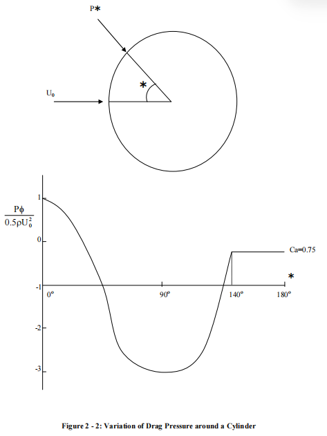
Shell or solid element models require more data. Such elements should be arranged into ASAS groups, each of which represents a ring of elements. The end co-ordinates, diameter and drag coefficients for each such ring are given in the AQWA-WAVE data. Rings are referenced by ASAS group number and assembled component name in the AQWA-WAVE data.
With two ends, a diameter and a drag coefficient, each ring can now be handled exactly as for the above tubes as far as the evaluation of distributed loads on the length of tubular. The distributed loads (which vary from end to end) now need to be assigned as pressure loads on to the wetted faces. Fortunately, there is ample literature to show the likely distribution of drag pressure around such a cylinder and a pressure distribution as illustrated in Figure 2 - 2is used. The co-ordinates of each node at each element of the ring is found and transformed relative to the start and end of the tube it represents. From this, a pressure can be derived according toFigure 2 - 1.
The drag loads on the tubular elements and the pressures on the elements of the rings are evaluated as above and are summed with incident/diffraction loads calculated in accordance with Section2.3, prior to being written to the output ASAS data file in the appropriate format.
It should be noted that the above treatment of the water surface elevation and linearisation of pressure loads is relatively simplistic. Excessive errors will occur if the element mesh is too coarse, particularly near the water surface. This should be remembered when meshing the model.
2.5 Inertial Loads
For floating structures, AQWA-WAVE writes body force and angular acceleration cards into the ASAS LOAD decks of all components containing massive elements. When ASAS is run, these will generate inertial loads to balance the pressure loads transferred from AQWA-LINE. If the ‘STAT’ option is selected, then static accelerations will be added, to balance the hydrostatic pressures which are included when this option is invoked. If the floating structure is in equilibrium in AQWA-LINE (as it should be) then the static acceleration will simply be the acceleration due to gravity.
For fixed structures, there is no dynamic acceleration and acceleration cards will only be output if the ‘STAT’ option is selected. In this case, the acceleration output is always the acceleration due to gravity. When ASAS is run, this will create inertial loads equal (in total) to the weight of the structure.
The user should note that there is no force balance in the case of fixed structures, since the reaction at the seabed is not modelled in AQWA-WAVE.
2.6 Units
Provision is made for the case where different units are used in AQWA and ASAS. AQWA-WAVE needs to know what the ASAS length units are and ASAS needs to know what the AQWA load units are. The user must supply this information in the AQWA-WAVE data file (see SCAL and UNIT commands in Section3.1.6), if the units are not consistent between AQWA and ASAS.
详细内容请见附件
免责声明:
本页面/内容部分素材来源于互联网公 开 信 息,旨在传递更多信息,不代表本平台立场。
版权归原作者或机构所有,如涉及侵权,请通过平台联系我们,我们将在核实后第一时间处理。
本平台对转载内容的真实性、准确性不作任何保证,用户需自行判断并承担使用风险。