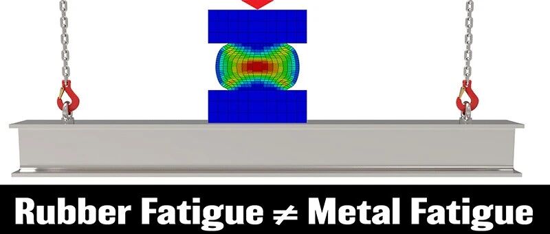
疲劳分析中要考虑的载荷情况可能非常长,并且可能涉及多个载荷轴。通常,载荷工况比通过直接时域有限元分析(FEA)计算的载荷工况要长得多。The load cases to be considered in fatigue an alysis can be very lengthy and can involve multiple load axes. Often, load cases are much longer than can be calculated via direct time-domain finite element an alysis (FEA).在金属疲劳分析中,线性叠加是一种广泛使用的技术,用于根据道路载荷生成应力应变历史[1],[2],[3]。当结构表现为线性时,这种方法是精确的和计算高效的,允许分析冗长的载荷信号。对于单轴问题,单个单元载荷情况的有限元(Fe)解根据输入载荷历史进行简单缩放。对于多轴问题,求解每个轴的单位载荷工况,然后根据输入载荷历史进行缩放和组合。In metal fatigue an alysis, linear superposition is a widely used technique to generate stress-strain history from road loads [1], [2], [3]. When structures behave linearly, this approach is accurate and computationally efficient, allowing the an alysis of lengthy load signals. For single axis problems, the finite element (FE) solution for a single unit load case is simply scaled according to the input load history. For multiaxial problems, unit load cases are solved for each of the axes, then scaled and combined according to the input load history.由于橡胶的1)非线性材料行为,2)非线性运动,3)非线性接触的可能性,线性叠加不能应用于橡胶疲劳分析。本文是研究橡胶疲劳分析程序与金属疲劳分析程序的不同之处的系列文章中的第二篇。在这里,我们介绍了Endurica EIETM(Endurica插值引擎)求解器,它是一种快速生成应力-应变历史的工具,用于在线性叠加失效的情况下进行疲劳分析。Due to rubber’s 1) nonlinear material behaviour, 2) nonlinear kinematics, and 3) the possibility of nonlinear contact, linear superposition cannot be applied to rubber fatigue an alysis. This article is the second in a series examining how rubber fatigue an alysis procedures differ from those used for metal fatigue. Here we present the Endurica EIETM (Endurica Interpolation Engine) solver, which is a tool for the rapid generation of stress-strain histories for fatigue an alysis in cases where linear superposition fails. 图1. 非线性图形在橡胶材料分析中的应用有多种方式,包括材料非线性、运动非线性和接触线性。当存在强非线性时,Endurica的EIE求解器为生成应力-应变历史提供了一种有效且准确的方法。Fig.1. Nonlinearity figures in the an alysis of rubbery materials in several ways including material nonlinearity, kinematic nonlinearity, and contact linearity. Endurica’s EIE solver provides an efficient and accurate method for generating stress-strain history when there is strong nonlinearity.01金属线性叠加法的简要评述Brief review of the linear superposition procedure for metals对于线性结构,力[F]和位移[U]之间的关系可以写成矩阵乘法,其中[K]是刚度矩阵。For linear structures, the relationship between forces [F] and displacements [u] can be written as a matrix multiplication where [k] is the stiffness matrix.[F] = [k][u]函数复合的结合性意味着将位移乘以标量a会产生成比例的较大力。The associative property of function composition means that multiplying the displacements by a scalar a produces proportionally larger forces.a[F] = [k](a[u])加法的分布性质是指由组合位移[u]和[v]产生的力系The distributive property of addition means that a force system resulting from combined displacements [u] and [v][F] = [k][u] +[k][v]也可以计算为can also be calculated as[F] = [k]([u] + [v])类似地,可以通过线性叠加来缩放和组合应力和应变场。多年来,工程师们一直在金属疲劳分析中使用这一原理,特别是在处理由现场记录的载荷-位移历史引起的多轴情况时。Similarly, stress and strain fields can be scaled and combined by linear superposition. Engineers have been using this principle for many years in metal fatigue an alysis, particularly for treating multiaxial cases arising from field-recorded oad-displacement histories.假设零件中的应力和应变场由单位载荷情况的线性组合产生,其中每个单位载荷情况的比例因子应用于给定输入通道对应的应力或应变场。The stress and strain fields in a part are assumed to result from a linear combination of unit load cases, where the scale factor for each unit load case is applied to the stress or strain field corresponding to a given input channel.例如,对于图2所示的梁,如果通道1是大小为a(t)的单位位移u,通道2是结构中其他位置的大小为β(t)的另一个单位位移v,则可以通过线性叠加恢复梁中所有点的应力和应变的整个历史。For example, for the beam shown in Fig.2, if channel 1 is the unit displacement u with magnitude a(t), and channel 2 is another unit displacement v elsewhere in the structure with magnitude β(t) , then the entire history of stress and strain at all points in the beam can be recovered by linear superposition.请注意,FE求解器只需为每个单位载荷工况生成一个与时间无关的解。完全通过比例因子a(t)和β(t)的时间变化来获得解的时间依赖性。这种极其有效的方法已在金属疲劳分析中使用多年。它允许快速分析由数百万个时间步长组成的完整道路载荷历史。Note that the FE solver only needs to produce a single time-independent solution for each unit load case. The time dependence of the solution is obtained entirely through the time variations of the scale factors a(t) and β(t). This extremely efficient method has been used for many years in metal fatigue an alysis. It allows rapid an alysis of complete road load histories consisting of millions of time steps. 图2. 在金属疲劳分析中,单一载荷情况下的线性叠加有限元解长期以来一直用于从道路载荷历史中生成应力应变历史。Fig.2. Linear superposition of single load case FE solutions has long been used to generate stress-strain histories from road load histories in metal fatigue an alysis.02Endurica EIETM:非线性情况下的载荷空间离散化和插值Endurica EIETM : load space discretization and interpolation for nonlinear cases解决非线性情况需要一种完全不同的方法。我们希望保留从预先计算的有限元解中有效构建应力-应变时间历程的优点。我们不是为每个输入通道预先计算单个单位载荷情况,而是从离散载荷空间中预先计算一组载荷情况。我们称这个集 合为地图。Solving the nonlinear case requires a completely different approach. We wish to retain the advantages of efficiently constructing stress-strain time histories from precomputed FE solutions. Instead of precomputing a single unit load case for each input channel, we precompute a set of load cases from a discretized load space. We call this set a map.图中载荷工况的数量必须足够,以便我们可以使用插值来获得图中任意点的非线性响应的合理近似值。图3显示了由x和z位移定义的两个通道的图。使用FE求解器如Ansys 或 LS-Dyna沿着蓝线所描绘的路径预先计算地图中的蓝点。一旦定义了映射,就可以从映射中预先计算的解中插入沿红线的应力-应变历史。The number of load cases in the map must be sufficient so that we can use interpolation to obtain an reasonable approximation of the nonlinear response at any point within the map. Fig.3 shows a map with two channels defined by x and z displacements. The blue points in the map are precalculated using an FE solver such as Ansys or LS-Dyna following the path traced by the blue line. Once the map is defined, the stress-strain history along the red line can be interpolated from the precomputed solutions in the map. 图3. 双通道映射离散化空间由x和z位移定义。蓝点表示预先计算了应力应变场的有限元解。蓝线表示解决方案路径,它定义了计算解决方案并将其存储在结果数据库中的顺序。红线表示可能的实际位移历史。红色路径上的点的应力-应变历史是通过从预先计算的图上的点进行插值获得的。Fig.3. Two-channel map discretizing a space defined by the x and z displacements. Blue dots represent FE solutions for which the stress-strain fields are precomputed. The blue line represents a solution path, which defines the order in which the solutions are computed and stored in the results database. The red line represents a possible actual displacement history. The stress-strain history for points on the red path is obtained by interpolation from points on the precomputed map.Endurica EIETM 是一种通用工具,用于创建和使用非线性映射来生成疲劳分析的应力-应变历史[4],[5]。EIE是Efficient Interpolation Engine(高效插值引擎)的缩写。EIE提供了一个简单的工作流程和强大的实用程序,用于创建和使用地图进行插值。它支持多达六个独立的输入通道。Endurica EIETM is a general purpose tool for creating and using non-linear maps to generate stress-strain histories for fatigue an alysis [4], [5]. EIE is an abbreviation for efficient interpolation engine. EIE provides a simple workflow and powerful utilities for creating and using maps for interpolation. It supports up to six independent input channels.整个EIE工作流程由三个主要步骤组成。第一步是创建地图。下一步是根据力或位移指定历史。请注意,任何可作为边界条件应用于有限元模型的量都可以设置为通道。最后一步是执行指定的插值。该过程为FE模型中的每个元素生成应变张量分量的时间历程。The entire EIE workflow consists of three main steps. The first step is to create a map. The next step is to specify your history in terms of forces or displacements. Note that any quantity that can be applied as a boundary condition to the FE model can be set up as a channel. The last step is to perform the specified interpolation. The process produces a time history of strain tensor components for each element in your FE model.地图创建过程包括四个步骤,如图4所示。首先,必须定义将用于指定历史的独立通道的数量。还必须指定映射类型。有几种类型可用,包括完全可自定义的地图。基于网格的地图通常适用于一维、二维和三维地图。对于高维映射,基于案例向量的映射通常是最方便的。The map creation process involves four steps, as shown in Fig.4. First, the number of independent channels that will be used to specify the history must be defined. The map type must also be specified. Several types are available, including a completely customizable map. Grid-based maps are often appropriate for one-, two- and three-dimensional maps. For higher dimensional maps, case vector-based maps are often the most convenient.一旦定义了映射类型,EIE就会生成解决方案路径。这些由列举的载荷状态组成,这些载荷状态应作为边界条件应用于有限元模型,以生成映射。根据映射类型,可以生成一个或多个路径。每条路径称为一个分支。对于每个分支,EIE都会编写一个具有适当边界条件历史的文件,这是生成地图所必需的。接下来,使用EIE的边界条件建立并执行有限元模型。最后,FE结果的数据库链接到地图定义中的相应分支。Once the map type has been defined, EIE generates solution paths. These consist of enumerated load states that should be applied as boundary conditions to the FE model to generate the map. One or more paths may be generated depending on map type. Each path is called a branch. For each branch, EIE writes a file with the appropriate boundary condition history, which is necessary for the generation of the map. Next, the FE model is set up and executed using EIE’s boundary conditions. Finally, the database of FE results is linked to the corresponding branch in the definition of the map.在这一点上,地图是完整的,并准备内插。请注意,当单位载荷情况解决方案被收集并定义为映射时,线性叠加可以作为EIE中的特殊情况实施。然而,一般来说,非线性映射将包含更多数量的求解步骤。At this point the map is complete and ready for interpolation. Note that linear superposition can be implemented as a special case in EIE when unit load case solutions are collected and defined as a map. In general, however, a non-linear map will contain a greater number of solution steps. 图4. 指定供 Endurica EIETM 使用的映射的步骤。Fig.4. Steps to specify a map for use by Endurica EIETM.指定载荷历史与选择包含每个输入通道的时间历史的文件一样简单。在文件中,每行表示一个时间步长,每列表示一个输入通道。EIE 支持 .csv 和 .rsp 格式,这两种格式都是常见的数据格式。图5显示了具有和位移的示例历史。请注意,历史中的位移范围不应超过预先计算的标测图的范围。尽管内插解可能相当精确,但非线性问题的外推可能非常危险和不准确。Specifying the load history is as simple as selecting a file containing the time history of each input channel. In the file, each row represents one time step and each column represents an input channel. EIE supports .csv and .rsp formats, both common data formats. Fig.5 shows an example history with and displacements. Note that the range of displacements in the history should not exceed the range of the precalculated map. Although interpolated solutions can be quite accurate, extrapolation for non-linear problems can be very risky and inaccurate. 图5. 插值的双通道位移历史示例。Fig.5. Example two-channel displacement history for interpolation.一旦指定了地图和历史,就可以开始插值。Endurica EIETM 支持多线程,这意味着插值计算可以在可用的CPU之间并行分布和执行。这使得插值速度非常快,并且可扩展到大型模型和冗长的历史。请注意,Endurica EIETM 生成的文件很大,因为它计算每个有限元的每个时间步长的应力和应变张量分量。因此,在运行Endurica EIETM 时,确保有足够的可用磁盘空间非常重要。Once the map and history are specified, interpolation can begin. Endurica EIETM supports multi-threading, meaning that interpolation calculations can be distributed and executed in parallel across available CPUs. This makes interpolating very fast and very scalable to large models and lengthy histories. Note that Endurica EIETM generates large files because it calculates stress and strain tensor components for each time step of each finite element. It is therefore important to ensure that you have sufficient disk space available when running Endurica EIETM.References[1.] R. W. Landgraf, “Applications of fatigue an alyses: transportation”, Fatigue ’87, vol. 3, pp. 1593–1610, 1987[2.] Moon, Seong-In et al, “Fatigue life evaluation of mechanical components using vibration fatigue a nalysis technique”, Journal of Mechanical Science and Technology, vol. 25, pp. 631–637, 2011.[3.] F. A. Conle and C. W. Mousseau, “Using vehicle dynamics simulations and finite-element results to generate fatigue life contours for chassis components”, International Journal of Fatigue, vol. 13(3), pp. 195–205, 1991.[4.] K. P. Barbash and W. V. Mars, “Critical plane an alysis of rubber bushing durability under road loads”, SAE Technical Paper No. 2016-01-0393, 2016.[5.] W. V. Mars, “Interpolation engine for an alysis of time-varying load data signals”. U.S. Patent 9, 645, 041, May 9, 2017.[6.] W. Mars, K. Barbash et al, “Durability of Elastomeric Bushings Computed from Track-Recorded Multi-Channel Road Load Input”, SAE Technical Paper No. 2024-01-2253, 2024.来源:Endurica