考虑重力荷载的二维/三维有限元分析C++编程实现

摘要: 采用三角形、四边形或六面体单元(网格),建立平面应变或三维弹性实体的有限元模型,通过能量原理推导出线性或二阶单元刚度的高斯积分表达式,组装出整体刚度矩阵,通过罚函数法处理边界条件,将重力荷载作为体积力考虑并且加入到总载荷列阵,得到有限元方程。 关键词:重力荷载(Gravity load),弹性实体(Elastic solid),平面应变(Plane strain),三维有限元,有限单元法(FEM),三角形单元(Triangle),四边形单元(Quadrilateral),六面体单元(Hexahedra),线性/二阶单元(Linear/Quadratic element),Lagrange形状函数,Serendipity形状函数,雅可比矩阵(Jacobian),能量原理,应变能,高斯积分,C++编程。 |
1. 引言
在有限元分析中,重力荷载的考虑与结构特性、分析类型及工程需求密切相关。以下是需考虑重力荷载的主要场景及依据:
本文在《六面体单元与弹性实体的三维有限元分析C++编程实现》的基础上,对程序算法进行改进,以考虑材料自身重力对结构静力分析的影响。具体做法如下:
单元材料特征向量prop增加第3个参数,即材料容重γ; 新增重力荷载向量gravlo,加入总荷载列阵,得到考虑材料自重的有限元方程; 可视化处理:将三维有限元方程求解前后的数据文件生成EnSight Gold格式。
2. 如何考虑重力荷载
2.1 等效集中荷载
文献[1]将分布荷载转换成等效集中荷载的分量,施加在总荷载列阵的相应位置(网格自由度),通常有以下几种情况:
单元节点处的集中荷载,直接加载到总荷载列阵; 非单元节点处的集中荷载,根据虚功原理转换成单元节点处的若干个等效荷载,然后逐个加载到总荷载列阵; 作用在结构表面的分布荷载(面积力),或者结构体积的分布荷载(体积力),根据虚功原理和形函数插值,分配给单元节点,得到各节点的等效集中荷载,然后逐个加载到总荷载列阵。
2.2 虚功原理与数值积分
重力荷载属于体积力,如何等效为单元节点的集中荷载?
假设单位体积的重力荷载为γ(材料重度),单元体积为dV,等效节点荷载为Pi(集中力),根据虚位移原理:
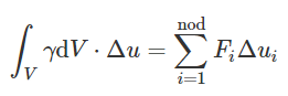
其中,V是重力荷载作用区域(网格单元),Δu是任意位置的虚位移,Δui是单元节点处的虚位移,nod为单元节点数,Ni为形函数,并且满足如下插值关系:
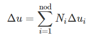
于是可以得到:
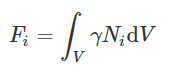
文献[1]附录详细推导得到网格单元的体积满足如下关系:

其中,det|J|是雅可比行列式,x-y-z是结构的整体坐标系,ξ-η-ζ是等参元的局部坐标系,将上式代入上上式得到:
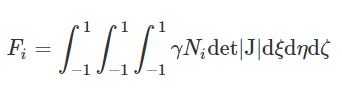
高斯积分法得到三重数值积分的通式为:

其中,f(ξ, η, ζ)是待积分函数,Wj是相应于高斯积分点(ξj, ηj, ζj)的加权系数,nip为高斯采样点的总数。于是得到:
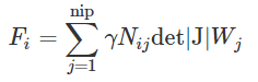
上式即为重力荷载在网格单元的第i个节点处的等效集中荷载Fi的高斯积分表达式,Nij是网格单元的第i个节点的形函数相应于第j个高斯积分点坐标的取值。
温馨提示:重力荷载竖直向下,其余方向分量为零。
3. 平衡方程与求解/回代
将Fi加载到整体结构的有限元方程[K]{U}={F}右端的总荷载列阵{F}相应的网格自由度,同时将边界条件整合到有限元方程,然后硅基生物就开始愉快地玩耍啦。
随后继续采用高斯积分法,将计算结果(总位移向量)回代到弹性力学的几何方程和本构方程,即可得到各单元积分点处的应变值和应力值,如下:
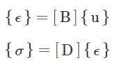
其中,{ε}为单位应变项,{σ}为单元应力项,{u}为单元位移列阵,[B]为应变-位移矩阵,[D]为应力-应变矩阵。
如果网格单元只考虑一个积分点的应变值和应力值的话,那就需要重置高斯积分点nip=1来找到各单元的等效中心点。
4. 程序设计(C++)
4.1. 网格生成
对于简单规则的几何体:自定义函数/子程序生成网格
通过mesh_size()和hexahedron_xz()自动生成三维空间网格; 通过mesh_size()和geom_rect()自动生成二维平面网格;
更普遍的做法:借助前处理软件/工具生成网格
然后直接读入各节点坐标、各单元节点编号、荷载和边界条件等信息。
4.2. 稀疏矩阵的处理
整体刚度矩阵[K]是带状分布的稀疏矩阵,且为对称正定矩阵。分两步处理:
将整体刚度矩阵(稀疏矩阵)进行Cholesky分解,于是该矩阵占用的内存减半、运算效率和数值稳定性都有显著提高; 将Cholesky分解得到的矩阵的非零项存储到一维向量空间kv,进一步节省存储空间和提高运算效率。
详情参照《弹性杆的有限元分析C++编程实现》第3.2节和第3.3节。
4.3. 后处理可视化
对于二维网格模型:自定义函数/子程序生成PostScript文件
通过mesh()提取几何数据,生成初始网格图*_mesh.ps和变形网格图*_dis.ps; 通过vecmsh()提取加载后的矢量场,生成位移向量图*_vec.ps; 利用GhostScript + GSview查看.ps图形。
对于三维网格模型:自定义函数/子程序生成EnSight Gold文件
通过mesh_ensi()和dis msh_ensi()提取数据,生成一系列EnSight Gold文件; 利用可视化工具ParaView查看EnSight Gold文件,进行FEM后处理。
4.4. 主程序流程图及C++源码
前面几篇文章,流程图过于详尽繁琐,俗称“太长不看版”。这次砍掉细枝末节,突出重点脉络,提纲挈领。
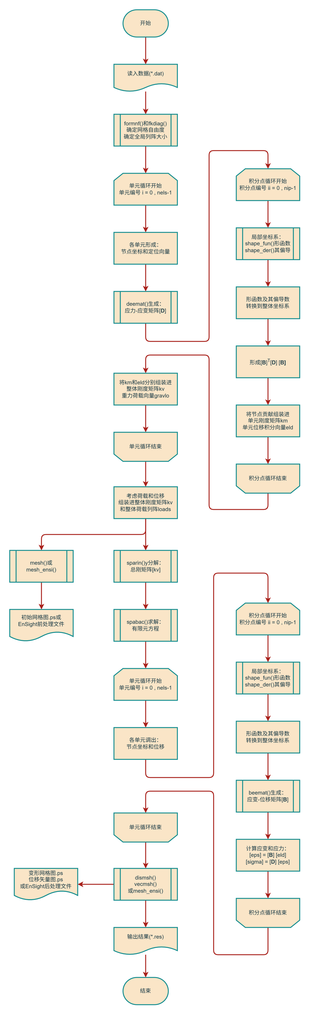
图1:主程序流程图
//===========================================================================// Program No.11 General two-(plane strain) or three-dimensional an alysis// of elastic solids(optional gravity loading).//===========================================================================using namespace std;int main() {int fixed_freedoms;//固定位移数int loaded_nodes;//受载节点数int ndim;//维数int ndof;//单元自由度int nels;//单元数int neq;//网格自由度int nip;//单元积分节点数int nn; //节点数int nod;//单元节点数int nodof;//节点自由度int nprops = 3;//材料特性数int np_types;//材料类型数int nr; //约束节点数int nst;//应力(应变)项数目double det;//雅可比矩阵行列式double penalty = 1.0e20; //罚因子string element;//单元类型string fin_name, fout_name;//读入文件名,写出文件名pair<string, string> argv;//文件名返回值//========================= input and initialisation =========================argv = getname();fin_name = argv.first;ifstream fin(fin_name, ios::in);fout_name = argv.second;ofstream fout(fout_name, ios::out);fin >> element >> nod;fin >> nels >> nn >> nip >> nodof >> nst >> ndim >> np_types;ndof = nod * nodof; //单元自由度vector<double> eld(ndof);//单元节点位移(单元自由度)vector<double> eps(nst);//应变项(应力/应变项数目)vector<int> etype(nels, 1);//单元特性类型向量(单元数)vector<double> fun(nod);//形函数(单元节点数)vector<int> g(ndof);//单元定位向量(单元自由度)vector<double> gc(ndim);//积分点坐标(维数)vector<int> num(nod);//单元节点编号向量(单元节点数)vector<double> sigma(nst);//应力项(应力/应变项数)vector<double> weights(nip);//数值积分加权系数(单元积分节点数)vector<vector<double> > bee(nst, vector<double>(ndof));//应变-位移矩阵(应力/应变项数, 单元自由度)vector<vector<double> > coord(nod, vector<double>(ndim));//单元节点坐标(单元节点数, 维数)vector<vector<double> > dee(nst, vector<double>(nst));//应力-应变矩阵(应力/应变项数, 应力/应变项数)vector<vector<double> > der(nod, vector<double>(ndim));//局部坐标下形函数的偏导数(单元节点数, 维数)vector<vector<double> > deriv(nod, vector<double>(ndim));//整体坐标下形函数的偏导数(单元节点数, 维数)vector<vector<double> > g_coord(nn, vector<double>(ndim));//所有单元的节点坐标(节点数, 维数)vector<vector<int> > g_g(nels, vector<int>(ndof));//总单元定位矩阵(单元数,单元自由度)vector<vector<int> > g_num(nels, vector<int>(nod));//总单元节点编号矩阵(单元数, 单元节点数)vector<vector<double> > jac(ndim, vector<double>(ndim));//雅可比矩阵(维数, 维数)vector<vector<double> > km(ndof, vector<double>(ndof));//单元刚度矩阵(单元自由度, 单元自由度)vector<vector<int> > nf(nn, vector<int>(nodof, 1));//节点自由度矩阵(节点数,节点自由度)vector<vector<double> > points(nip, vector<double>(ndim));//单元积分点坐标(单元的积分点数, 维数)vector<vector<double> > prop(np_types, vector<double>(nprops));//单元特征矩阵(材料类型数, 材料特性数)for (int i = 0; i < np_types; i++) {//从文件中读入:单元特征矩阵for (int j = 0; j < nprops; j++)fin >> prop[i][j];}if (np_types > 1) {//从文件中读入:单元特性类型向量for (int i = 0; i < nels; i++)fin >> etype[i];}for (int i = 0; i < nn; i++) {for (int j = 0; j < ndim; j++) {fin >> g_coord[i][j]; //从文件中读入:各节点的坐标}}for (int i = 0; i < nels; i++) {for (int j = 0; j < nod; j++) {fin >> g_num[i][j];//从文件中读入:各单元的节点编号}}fin >> nr;//从文件中读入:约束节点数vector<int> k1(nr);//约束节点编号向量(约束节点数)if (nr > 0) {//从文件中读入:约束节点编号及自由度for (int i = 0; i < nr; i++) {fin >> k1[i];for (int j = 0; j < nodof; j++) {int m = k1[i] - 1;fin >> nf[m][j];}}}auto result0 = formnf(nf);neq = result0.first;//返回:网格自由度数目nf = result0.second;//生成:节点自由度矩阵vector<int> kdiag(neq);//对角项局部向量(网格自由度)vector<double> loads(neq);//总体荷载/位移向量(网格自由度)vector<double> gravlo(neq);//总体重力荷载向量(网格自由度)//=============== loop the elements to find global array sizes ================for (int i = 0; i < nels; i++) {num = g_num[i];//第i个单元的节点编号向量g = num_to_g(num, nf);//生成:单元定位向量kdiag = fkdiag(g, kdiag);//生成:对角项局部向量g_g[i] = g;//第i个单元的定位向量}for (int i = 1; i < neq; i++)//生成:对角项局部向量kdiag[i] = kdiag[i] + kdiag[i - 1];fout << "There are " << neq << " equations and the skyline storage is "<< kdiag[neq - 1] << endl;cout << "There are " << neq << " equations and the skyline storage is "<< kdiag[neq - 1] << endl;//================ element stiffness integration and assembly ================vector<double> kv(kdiag[neq - 1]);//初始化:整体刚度向量auto result1 = sample(element, nip, ndim);points = result1.first;//生成:单元积分点坐标weights = result1.second;//生成:加权系数for (int i = 0; i < nels; i++) {int m = etype[i] - 1;dee = deemat(prop[m][0], prop[m][1], nst); //生成:应力-应变矩阵[D]num = g_num[i];//第i个单元的节点编号向量g = g_g[i];//第i个单元的定位向量for (int j = 0; j < nod; j++) {int k = num[j] - 1;coord[j] = g_coord[k];//第i个单元的节点坐标矩阵}fill(eld.begin(), eld.end(), 0.0);fill(km.begin(), km.end(), vector<double>(ndof, 0.0));vector<vector<double> > btdb(ndof, vector<double>(ndof, 0.0));for (int ii = 0; ii < nip; ii++) {fun = shape_fun(ii, nod, points);//生成:形函数der = shape_der(ii, nod, points);//生成:局部坐标下形函数的偏导数jac = matmul(transpose(der), coord); //生成:雅可比矩阵det = determinant(jac);//生成:雅可比矩阵行列式jac = invert(jac);//生成:雅可比矩阵的逆deriv = matmul(der, jac);//生成:整体坐标下形函数的偏导数bee = beemat(nst, ndof, deriv);//生成:应变-位移矩阵[B]btdb = matmul(matmul(transpose(bee), dee), bee);for (int jj = 0; jj < ndof; jj++) {for (int kk = 0; kk < ndof; kk++)btdb[jj][kk] *= det * weights[ii];}for (int jj = 0; jj < ndof; jj++) {for (int kk = 0; kk < ndof; kk++)km[jj][kk] += btdb[jj][kk];}//生成:单元刚度矩阵for (int jj = nodof - 1; jj < ndof; jj += nodof)eld[jj] += fun[jj / nodof] * det * weights[ii];}kv = fsparv(km, g, kdiag, kv);//生成:整体刚度矩阵for (int k = nodof - 1; k < ndof; k += nodof) {if (g[k]) {int n = g[k] - 1;gravlo[n] -= eld[k] * prop[m][2];//生成:总体网格的重力荷载向量}}}fin >> loaded_nodes;//从文件读入:受载节点数vector<int> k2(loaded_nodes);//初始化:受载节点编号向量if (loaded_nodes) {//从文件读入:受载节点编号,相应荷载向量for (int i = 0; i < loaded_nodes; i++) {fin >> k2[i];int m1 = k2[i] - 1;for (int j = 0; j < nodof; j++) {if (nf[m1][j]) {int m2 = nf[m1][j] - 1;fin >> loads[m2];}elsefin.ignore(5);}}}for (int k = 0; k < neq; k++)loads[k] += gravlo[k];//考虑重力荷载if (ndim == 3)//生成:三维模型的前处理文件Ensight Gold格式mesh_ensi(fin_name, g_coord, g_num, element, etype, nf, loads, 1, 1, 0.0, true);elsemesh(g_coord, g_num, fin_name);//生成:二维模型的初始网格图(*_mesh.ps)fin >> fixed_freedoms;//从文件读入:固定位移的数量if (fixed_freedoms) {vector<int> node(fixed_freedoms);//固定节点向量vector<int> no(fixed_freedoms);//固定自由度编号向量vector<int> sense(fixed_freedoms);//固定自由度的检测向量vector<double> value(fixed_freedoms);//给定位移向量for (int i = 0; i < fixed_freedoms; i++) {fin >> node[i] >> sense[i] >> value[i];int j = node[i] - 1;int k = sense[i] - 1;no[i] = nf[j][k];int m = no[i] - 1;int n = kdiag[m] - 1;kv[n] += penalty;loads[m] = kv[n] * value[i];}}//============================ equation solution =============================kv = sparin(kv, kdiag);//整体刚度矩阵kv的Cholesky三角分解形式loads = spabac(kv, loads, kdiag);//求解有限元方程,得到总体 位移向量if (ndim == 3) {fout << endl << " Node x-disp y-disp z-disp" << endl;cout << endl << " Node x-disp y-disp z-disp" << endl;}else {fout << endl << " Node x-disp y-disp" << endl;cout << endl << " Node x-disp y-disp" << endl;}for (int i = 0; i < nn; i++) {fout << setw(4) << i + 1;cout << setw(4) << i + 1;for (int j = 0; j < nodof; j++) {if (nf[i][j]) {int k = nf[i][j] - 1;fout << setw(14) << scientific << setprecision(4) << loads[k];cout << setw(14) << scientific << setprecision(4) << loads[k];}else {fout << " 0.0000e+00";cout << " 0.0000e+00";}}fout << endl;cout << endl;}//================ recover stresses at element Gauss - points ================//nip = 1;//points.resize(nip, vector<double>(ndim));//weights.resize(nip);//auto result2 = sample(element, nip, ndim);//points = result2.first;//生成:单元积分点坐标//weights = result2.second;//生成:加权系数fout << endl << " The integration point ( nip = " << nip << " ) stresses are:" << endl;cout << endl << " The integration point ( nip = " << nip << " ) stresses are:" << endl;if (ndim == 3) {fout << " Element x-coord sig_x tau_xy" << endl;cout << " Element x-coord sig_x tau_xy" << endl;fout << " y-coord sig_y tau_yz" << endl;cout << " y-coord sig_y tau_yz" << endl;fout << " z-coord sig_z tau_zx" << endl;cout << " z-coord sig_z tau_zx" << endl;}else {fout << " Element x-coord y-coord sig_x sig_y tau_xy" << endl;cout << " Element x-coord y-coord sig_x sig_y tau_xy" << endl;}for (int i = 0; i < nels; i++) {if (np_types > 1) {int m = etype[i] - 1;dee = deemat(prop[m][0], prop[m][1], nst);}//生成:应力-应变矩阵[D]elsedee = deemat(prop[0][0], prop[0][1], nst);num = g_num[i];//生成:第i个单元的节点编号向量for (int j = 0; j < nod; j++) {int k = num[j] - 1;coord[j] = g_coord[k];//生成:第i个单元的节点坐标矩阵}g = g_g[i];//生成:第i个单元的定位向量for (int k = 0; k < ndof; k++) {if (g[k]) {int m = g[k] - 1;eld[k] = loads[m];//生成:第i个单元的位移向量}elseeld[k] = 0.0;}for (int ii = 0; ii < nip; ii++) {fout << setw(4) << i + 1;cout << setw(4) << i + 1;fun = shape_fun(ii, nod, points);//生成:形函数der = shape_der(ii, nod, points);//生成:局部坐标下形函数的偏导数gc = matmul(fun, coord);//生成:积分点坐标jac = matmul(transpose(der), coord); //生成:雅可比矩阵jac = invert(jac);//生成:雅可比矩阵的逆deriv = matmul(der, jac);//生成:整体坐标下形函数的偏导数bee = beemat(nst, ndof, deriv);//生成:应变-位移矩阵[B]eps = matmul(bee, eld);//生成:单元应变向量sigma = matmul(dee, eps);//生成:单元应力向量if (ndim == 3) {fout << setw(14) << scientific << setprecision(4) << gc[0]<< setw(14) << scientific << setprecision(4) << sigma[0]<< setw(14) << scientific << setprecision(4) << sigma[3] << endl;cout << setw(14) << scientific << setprecision(4) << gc[0]<< setw(14) << scientific << setprecision(4) << sigma[0]<< setw(14) << scientific << setprecision(4) << sigma[3] << endl;fout << " " << setw(14) << scientific << setprecision(4) << gc[1]<< setw(14) << scientific << setprecision(4) << sigma[1]<< setw(14) << scientific << setprecision(4) << sigma[4] << endl;cout << " " << setw(14) << scientific << setprecision(4) << gc[1]<< setw(14) << scientific << setprecision(4) << sigma[1]<< setw(14) << scientific << setprecision(4) << sigma[4] << endl;fout << " " << setw(14) << scientific << setprecision(4) << gc[2]<< setw(14) << scientific << setprecision(4) << sigma[2]<< setw(14) << scientific << setprecision(4) << sigma[5] << endl;cout << " " << setw(14) << scientific << setprecision(4) << gc[2]<< setw(14) << scientific << setprecision(4) << sigma[2]<< setw(14) << scientific << setprecision(4) << sigma[5] << endl;}else {for (int n = 0; n < ndim; n++) {fout << setw(14) << scientific << setprecision(4) << gc[n];cout << setw(14) << scientific << setprecision(4) << gc[n];}for (int n = 0; n < nst; n++) {fout << setw(14) << scientific << setprecision(4) << sigma[n];cout << setw(14) << scientific << setprecision(4) << sigma[n];}fout << endl;cout << endl;}}}if (ndim == 3)dis msh_ensi(fin_name, 1, nf, loads);//生成:三维模型的后处理文件Ensight Gold格式else {dis msh(loads, nf, 0.05, g_coord, g_num, fin_name);//生成:二维模型的变形网格图(*_dis.ps)vecmsh(loads, nf, 0.05, 0.1, g_coord, g_num, fin_name);//生成:二维模型的位移矢量图(*_vec.ps)}fin.close();fout.close();}
主程序可用于二维/三维有限元静力分析,三角形/四边形/六面体单元(网格),考虑外加荷载和边界条件,重力荷载可选。涉及到的子程序/函数有7类:
高斯积分法与形函数:sample(),shape_fun(),shape_der(); 单元刚度矩阵:beemat(),deemat(); 矩阵计算:transpose(),matmul(),determinant(),invert(); 前后处理可视化:mesh(),dis msh(),vecmsh(),mesh_ensi(),dis msh_ensi(); 单元定位与总刚集成(稀疏矩阵):num_to_g(),fkdiag(),formnf(),fsparv(); 矩阵分解与有限元方程求解:sparin(),spabac(); 文件流与命名:getname()。
第1~2类子程序/函数源码可参照以下4篇文章:
矩形薄板的有限元分析C++编程实现 3节点三角形单元(T3)与二维有限元分析C++编程实现 四边形单元(Q4/Q8)与轴对称弹性实体的非对称分析的半解析有限元方法C++编程实现 六面体单元与弹性实体的三维有限元分析C++编程实现
第3类子程序/函数源码可参照以下1篇文章:
矩阵转置/求逆/点乘、行列式求值与C++面向对象编程
第4类子程序/函数源码可参照以下4篇文章:
PostScript编程与FEM网格生成→加载变形的可视化 PostScript编程与FEM位移矢量场的可视化 从数据提取到可视化:使用EnSight与ParaView进行FEM后处理(上篇) 从数据提取到可视化:使用EnSight与ParaView进行FEM后处理(下篇)
第5~7类子程序/函数源码可参照以下1篇文章:
弹性杆的有限元分析C++编程实现
5. 数值案例
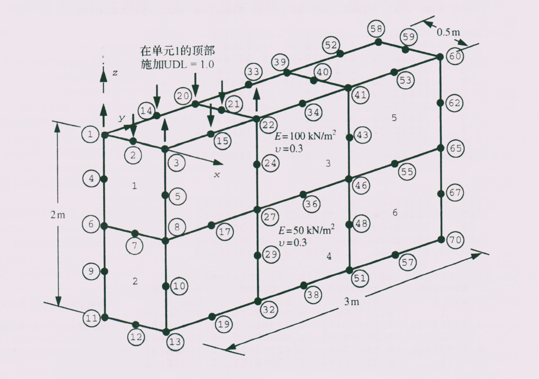
图2:立方弹性实体
上图所示的立方弹性实体,尺寸0.5×3.0×2.0m³,两种材料的弹性模量不同,密度均为1.0×10³kg/m³,采用二阶六面体减缩积分单元,划分成6个网格,共计70个节点。网格1的上表面承受1.0kN/m²的均布压力,该面积力折算成①②③⑭⑮⑳㉑㉒这8个节点等效集中荷载,底面铰支座。输入数据*.dat文件的相关内容如下:
=====================================
  数值案例:立方弹性实体结构的数据输入
=====================================

单元类型element    单元节点数nod
  hexahedron          20

单元数nels  节点数nn  单元积分点nip  节点自由度nodof
    6          70         8              3

应力/应变项数nst    维数ndim    材料类型数np_types
    6                  3              2

单元特征值prop(弹性模量e, 泊松比v,容重γ)
100.0e3  0.3  9.81e3
 50.0e3  0.3  9.81e3

单元特性类型etype
1   2   1   2   1   2

整体节点坐标g_coord
0.000.000.00
0.25 0.00 0.00
0.50 0.00 0.00
0.00 0.00   -0.50
0.50 0.00   -0.50
0.00 0.00   -1.00
0.25 0.00   -1.00
0.50 0.00   -1.00
0.00 0.00   -1.50
0.50 0.00   -1.50
...
0.00 3.00   -0.50
0.50 3.00   -0.50
0.00 3.00   -1.00
0.25 3.00   -1.00
0.50 3.00   -1.00
0.00 3.00   -1.50
0.50 3.00   -1.50
0.00 3.00   -2.00
0.25 3.00   -2.00
0.50 3.00   -2.00

单元节点编号g_num
 6  4  1  2  3  5  8  7 16 14 15 17 25 23 20 21 22 24 27 26
11  9  6  7  8 10 13 12 18 16 17 19 30 28 25 26 27 29 32 31
25 23 20 21 22 24 27 26 35 33 34 36 44 42 39 40 41 43 46 45
30 28 25 26 27 29 32 31 37 35 36 38 49 47 44 45 46 48 51 50
44 42 39 40 41 43 46 45 54 52 53 55 63 61 58 59 60 62 65 64
49 47 44 45 46 48 51 50 56 54 55 57 68 66 63 64 65 67 70 69

约束节点数nr
约束节点编号k1与相应的自由度nf
18
11 0 0 0  12 0 0 0  13 0 0 0  18 0 0 0  19 0 0 0
30 0 0 0  31 0 0 0  32 0 0 0  37 0 0 0  38 0 0 0
49 0 0 0  50 0 0 0  51 0 0 0  56 0 0 0  57 0 0 0
68 0 0 0  69 0 0 0  70 0 0 0

给定位移数fixed_freedoms
节点编号node与相应的位移值value
8
 1  0.0  0.0  0.0417e3    2  0.0  0.0 -0.1667e3    3  0.0  0.0  0.0417e3
14  0.0  0.0 -0.1667e3   15  0.0  0.0 -0.1667e3   20  0.0  0.0  0.0417e3
21  0.0  0.0 -0.1667e3   22  0.0  0.0  0.0417e3

给定位移数fixed_freedoms
0
采用本文算法程序读入*.dat文件,得到计算结果*.res如下。
====================================================
  数值案例:立方弹性实体结构的节点位移和单元积分点应力
====================================================

There are 156 equations and the skyline storage is 6594

  Node    x-disp        y-disp        z-disp
   1    5.4733e-03   -2.3283e-02   -3.3709e-01
   2   -8.9368e-15   -2.3622e-02   -3.4014e-01
   3   -5.4733e-03   -2.3283e-02   -3.3709e-01
   4   -7.2285e-03   -3.9747e-02   -3.2099e-01
   5    7.2285e-03   -3.9747e-02   -3.2099e-01
   6    2.7202e-03   -5.7007e-02   -2.8255e-01
   7   -2.8657e-15   -5.6394e-02   -2.8317e-01
   8   -2.7202e-03   -5.7007e-02   -2.8255e-01
   9   -3.4802e-02   -7.5465e-02   -1.6300e-01
  10    3.4802e-02   -7.5465e-02   -1.6300e-01
  ..
  61   -6.4056e-03    1.9508e-02   -2.8980e-01
  62    6.4056e-03    1.9508e-02   -2.8980e-01
  63    3.3605e-03    4.5983e-02   -2.5716e-01
  64    3.4284e-15    4.5247e-02   -2.5763e-01
  65   -3.3605e-03    4.5983e-02   -2.5716e-01
  66   -3.1942e-02    6.9985e-02   -1.5055e-01
  67    3.1942e-02    6.9985e-02   -1.5055e-01
  68    0.0000e+00    0.0000e+00    0.0000e+00
  69    0.0000e+00    0.0000e+00    0.0000e+00
  70    0.0000e+00    0.0000e+00    0.0000e+00

 The integration point ( nip = 8 ) stresses are:
 Element  x-coord       sig_x         tau_xy
          y-coord       sig_y         tau_yz
          z-coord       sig_z         tau_zx
   1    3.9434e-01    7.8756e+01    5.6835e+00
        7.8868e-01    5.4098e+02    2.7211e+02
       -2.1132e-01   -2.7041e+03   -1.5338e+02
   1    3.9434e-01   -6.0197e+02   -2.6567e+01
        7.8868e-01   -2.2980e+02    5.6863e+02
       -7.8868e-01   -8.6752e+03    5.9904e+02
   1    3.9434e-01    2.2661e+01    7.3173e+00
        2.1132e-01   -1.2000e+02    3.9307e+01
       -2.1132e-01   -3.1145e+03   -1.8516e+02
        ......
   2    3.9434e-01    1.0599e+03    2.0614e+01
        7.8868e-01   -8.7683e+02    1.3356e+02
       -1.2113e+00   -1.2751e+04   -8.1983e+02
   2    3.9434e-01   -1.6090e+03    1.2767e+01
        7.8868e-01   -4.0715e+03   -9.0955e+02
       -1.7887e+00   -1.7999e+04    9.9989e+02
        ......
   3    3.9434e-01   -1.0589e+01   -4.4650e-01
        1.7887e+00    8.7300e+02   -1.2106e+02
       -2.1132e-01   -2.1669e+03   -1.5222e+02
        ......
   6    1.0566e-01    1.0314e+03    2.6876e+01
        2.2113e+00   -8.8741e+02   -1.5534e+02
       -1.2113e+00   -1.2102e+04    8.0076e+02
   6    1.0566e-01   -1.9448e+03    2.3957e+01
        2.7887e+00   -4.0228e+03    2.4468e+03
       -1.7887e+00   -1.7400e+04   -8.7048e+02
   6    1.0566e-01   -1.5809e+03    2.3994e+01
        2.2113e+00   -4.0111e+03    9.3366e+02
       -1.7887e+00   -1.7395e+04   -9.6416e+02
采用本文算法自动生成EnSight Gold后处理文件,通过ParaView查看位移云图如图3。这配色比例,像不像西瓜?给炎炎夏日带来清凉。
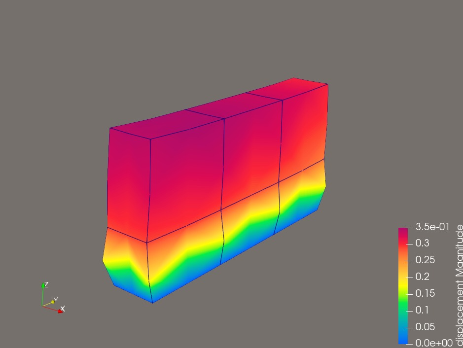
图3:位移云图-本文算法
如果不考虑重力荷载,也就是材料容重置零,那么位移云图如图4所示:
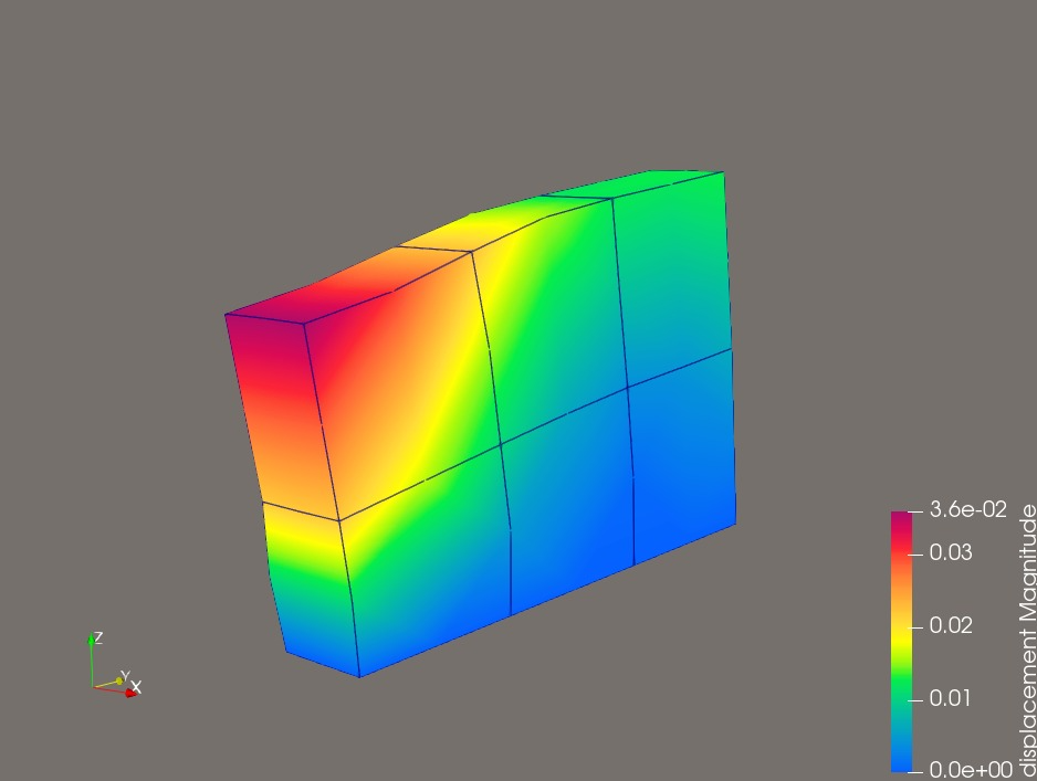
图4:位移云图-本文算法-不考虑重力荷载
足以说明,此时重力荷载是不容忽视的。
接下来用ABAQUS三维有限元模型进行对比,二阶六面体减缩积分单元C3D20R,划分成6个网格,共计70个节点。施加表面力,考虑材料自重,底面铰支座。
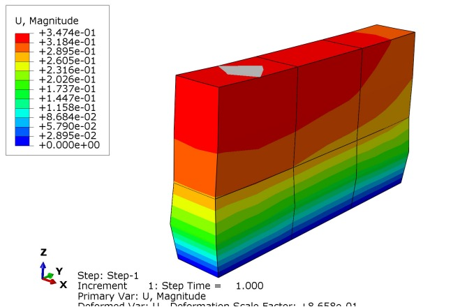
图5:位移云图-ABAQUS验算
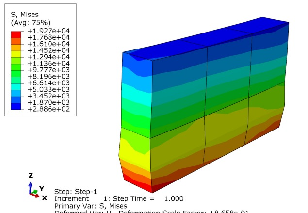
图6:应力云图-ABAQUS验算
图3和图5位移云图对比,基本一致。同时对比本文算法和ABAQUS验算的节点位移和单元积分点应力,差距不超过0.4%,除了极个别差距接近0.8%。差距较大的极个别节点,位于立方弹性体下层网格,其x方向的位移和应力均大于ABAQUS计算结果,换用压缩模量较大的材料是不是更合理?或者有什么黑科技?
6. 讨论
本文采用虚功原理推导出重力荷载(体积力)在网格节点的等效集中荷载。单元刚度矩阵是采用最小势能原理推导出来的,也可以采用伽辽金方法(Galerkin)。如何打通结构力学和弹塑性力学的任督二脉?能量原理足矣。记得当年结构力学教材将其列为选修内容,没有能量原理学个寂寞啊。
b站李老师《能量原理与变分法》讲的不错,80P将近11小时,第一遍看不懂,第二遍大受震撼;而且声音很好听,谦谦君子,温润如玉,不由得想到乌尔善电影《封shen第yi部:朝歌风云》里的伯邑考。大家有兴趣可以去“李老师的云课堂”哦。
参考文献:
[1]: T. R. Chandrupatla, A. D. Belegundu 著. 曾攀, 雷丽萍 译. 工程中的有限元法(原书第4版)[M]. 北京:机械工业出版社, 2021 [2]: 龙驭球, 包世华, 袁驷 主编. 结构力学I——基础教程(第4版)[M]. 北京: 高等教育出版社, 2018 [3]: I. M. S mith, D. V. Griffiths, L. Margetts 著. 张新春, 慈铁军, 范伟丽 等译. 有限元方法编程(原书第5版)[M]. 北京: 电子工业出版社, 2017