
首页/文章/ 详情

Deform Inverse Heat Transfer Wizard Lab(逆向热传模块向导)

2月前浏览932

Deform Inverse Heat Transfer Wizard Lab(逆向热传模块向导)

摘要:本文详细介绍 DEFORM 逆向热传导向导(Inverse Heat Transfer Wizard)的完整操作流程,用于基于实测温度数据反演工件与介质间的换热系数。操作步骤包括新建问题、单位设置、几何导入、网格划分、材料定义、初始温度设定、测温点布置、导入热历史数据、划分换热区域、定义温度相关换热系数函数、仿真控制、优化参数设置、启动优化计算及结果查看。系统通过优化算法拟合出各区域 HTC–温度关系,对比模拟与实测温度曲线验证精度,适用于淬火、冷却等工艺的热边界条件识别,操作规范、工程实用性强。


INVERSE HEAT TRANSFER WIZARD LAB

1.Starting a new problem 1

2.Set unit system 1

3.Import geometry 2

4.Generate mesh 2

5.Material definition 3

6.Initial temperature 4

7.Temperature Measurement Points 5

8.Thermal history 6

9.Heat transfer zones 6

10.Heat transfer coefficient function definition 7

11.Simulation control 8

12.Optimization control 9

13.Optimization 9

14.Optimization results 10


Problem Summary:

This lab will demonstrate how to use the Inverse Heat Transfer Wizard to determine heat transfer coefficients of between workpiece and a medium during a heat transfer process. Temperature measurement data are needed. Heat transfer coefficients can be functions of temperature or time. Multiple zones of heat-transfer coefficients are assigned to the workpiece. 

1.Starting a new problem

Start a new Inverse Heat Transfer Wizard problem with problem ID BAR INVHEAT. You can do so by clicking the “New problem” button and choose “Inverse Heat”. Alternatively, you can right click on the directory tree to create an empty directory and then click “Inverse Heat” on the right side of the main window. 
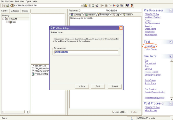
image.png


2. Set unit system

You should see a window as below, choose "English" for Unit System. Click"Next".

                    DEFORM™-Inverse Heat Transfer Wizard Lab
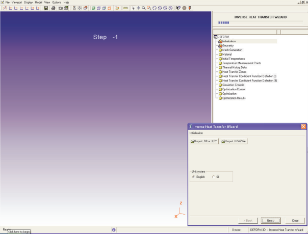
image.png

3.Import geometry

In page “Geometry”, choose “import from a geometry, KEY, or DB file” and click “Next”. Import geometry file “BAR INVHEAT.STL” from labs/ directory. 


4.Generate mesh

In page “Mesh Generation”, use 2000 for unstructured mesh. Click “Next”. 

                     DEFORM™-Inverse Heat Transfer Wizard Lab
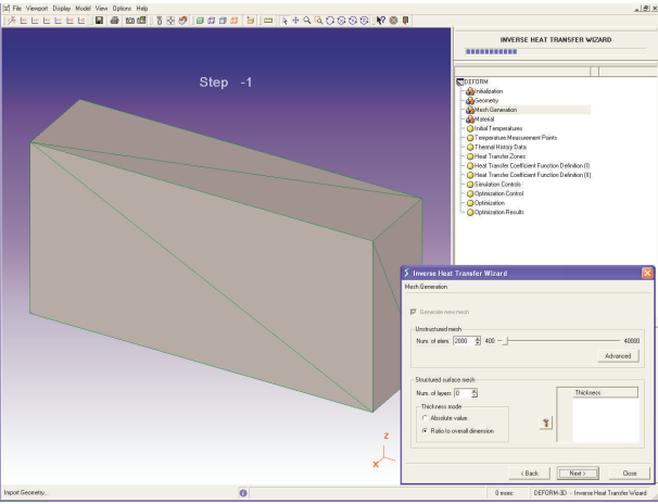
image.png


5.Material definition

In page “Material”, choose “Load from material library” and click “Next”. Choose material "AISI-1015[70-2000F(20-1100C)]" from the "Steel" category. 

                          DEFORM™-Inverse Heat Transfer Wizard Lab
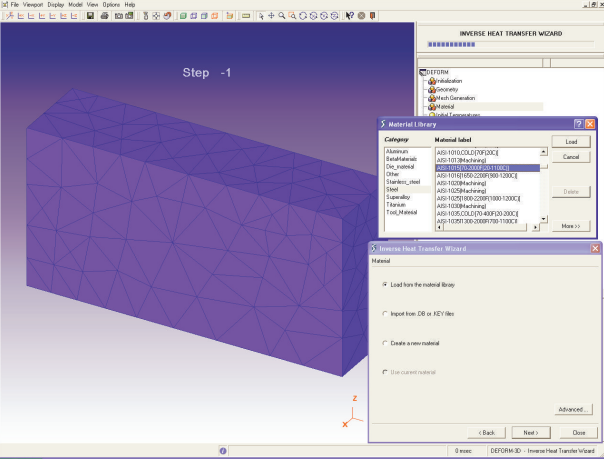
image.png


6.Initial temperature

In page “Initial temperature", for workpiece choose "Uniform" and set 1575 F. For Environment, choose constant 150F. 
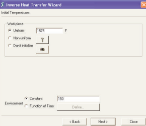
image.pngDEFORM™-Inverse Heat Transfer Wizard Lab

7. Temperature Measurement Points

In “Temperature Measurement Points” page, click “Add” button three times. Specify the measurement point coordinates by first selecting the corresponding rows on the table and then clicking on the object. Pick the points approximately as indicated in the graph: for the first point, pick a point near (1.249, 4.5, 4.5). For the second point, pick a point near (1.249, 0, 0.5). The third point is near (1.249, -4.9, 2.5). (Of course, you can also input this coordinates directly into the table.) Click “Next”.
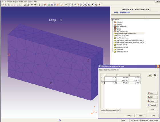
image.png

8.Thermal history

In “Thermal History” page, click the "Load thermal history from a file" button and load the file “BAR_INVHEAT_Thermal_History.DAT” in directory /labs. Click “Apply” to see the graphs. Input 506 seconds for “Process End Time”. Click “Next”. 
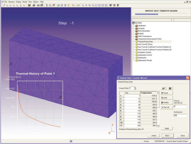
image.png

                          DEFORM™-Inverse Heat Transfer Wizard Lab

9.Heat transfer zones

In page “Heat transfer zones”, click “Add” twice. To define each heat transfer zone, first select the appropriate row in the table and then pick surfaces on the object. (You may need to use in the picking dialog at the lower-left corner in order to achieve ideal picking results.) As indicated in the graph below, pick the top (long narrow face) and end face surfaces for Zone #1, the bottom (the other long narrow face) surface for Zone #2. 

Note that the symmetric planes should not be included in any heat transfer zone. In this set up, there are two symmetric planes, one of which is where the three  temperature-measurement points are located. The other symmetric plane is the "minimum-Y" plane, which is near point #3. Click "Next".
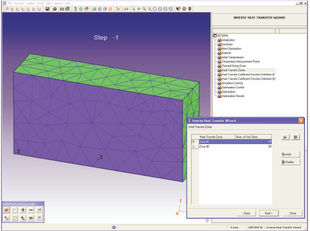
image.png

10.Heat transfer coefficient function definition

In page “Heat transfer coefficient function definition (I)”, set heat transfer coefficient as a function of temperature. This function will be defined by HTC values at six different temperatures: 100, 400, 700, 1000, 1300 and 1600F. Therefore, toggle on “Initialize functions” and input "6" for “Number of control points”. In table “Control points”, input the temperatures accordingly. The default initial guess, lower and upper bounds are fine. Click “Next”. 
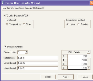
image.png

In page “Heat transfer coefficient function definition (II)”, all defaults are fine. Click “Next”. 
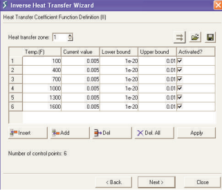
image.pngDEFORM™-Inverse Heat Transfer Wizard Lab

11.Simulation control

In “Simulation Control” page, use step definition “Auto”, and set “Temperature change per step” to 1.0. Click “Next”. 
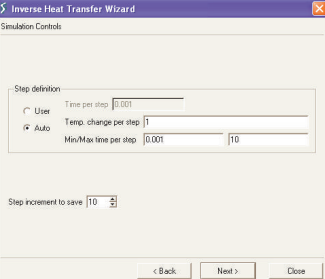
 image.png

12.Optimization control

In “Optimization Control” page, all default settings are fine, so click “Next”.
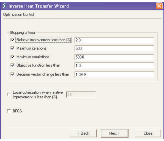
 image.png

13. Optimization

In “Optimization” page, click “Check Data” to check whether all data are valid. If so, click “Start”. The optimization may take a few hours depending on the speed of your computer. (5 hours on a Pentium IV 2.0Ghz CPU.) You may activate the background command prompt to see program output. 

After the first iteration is completed, you can see the history of the objective function on the left. During optimization, you can also view current optimization results by going to the next page. 
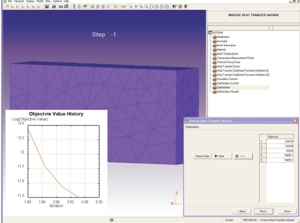
image.png


14.Optimization results

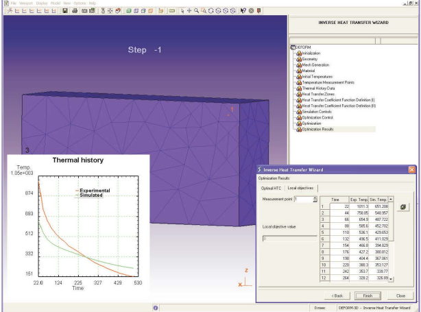
In “Optimization Result” page, you can view the currently best heat transfer coefficients and compare the simulated thermal history with the measured thermal history. You can save the optimization results if necessary. Please note that the convergence of optimization procedures greatly depends upon the nature of the data used. For example when the temperature measurement points are on the surface, indicating at least one heat transfer zone per measurement point aids solution convergence. Similarly when the measured thermal data is a function of time, defining time dependent convection heat transfer coefficient can lead to faster convergence. Other factors that can influence the convergence include, spacing of the temperature data points to accurately represent the gradient information in the measured data and good initial guess if any that can be indicated to the system. 
92d2ae1a6796bbbb17fab03ac305f6e4.png


免责声明:

本页面/内容部分素材来源于互联网公 开 信 息,旨在传递更多信息,不代表本平台立场。

版权归原作者或机构所有,如涉及侵权,请通过平台联系我们,我们将在核实后第一时间处理。

本平台对转载内容的真实性、准确性不作任何保证,用户需自行判断并承担使用风险。

ACTSystemDeformCONVERGEUM材料NVH控制
著作权归作者所有,欢迎分享,未经许可,不得转载
首次发布时间:2026-06-02
最近编辑:2月前
仿真支持爱好者
在仿真的路上越走越远
获赞 333粉丝 21文章 318课程 0
点赞
收藏
作者推荐

基于新数据的氢燃烧详细动力学模型更新

N15-基于新数据的氢燃烧详细动力学模型更新([New+good]An Updated Comprehensive Kinetic Model of Hydrogen Combustion)摘要:本文基于 Mueller 等人的氢氧燃烧机理,结合最新热力学与动力学数据,构建了更新版氢气燃烧详细动力学模型。模型更新了 OH 生成焓、H+O₂支链反应与 H+O₂(+M) 三体反应速率,修正 H+OH+M 反应参数以提升高压火焰预测精度。经激波管点火延迟、变压流动反应器组分分布、1–20 atm 层流火焰速度及稳焰火焰组分验证,在 298–3000 K、0.3–87 atm、当量比 0.25–5.0 宽工况下与实验高度吻合。该模型适用 CHEMKIN-II,可精准预测氢氧燃烧特性,为烃类燃烧机理提供可靠子模型基础。ABSTRACT: A comprehensively tested H2/O2 chemical kinetic mechanis m based on the work ofMueller et al. [ 1 ] and recently published kinetic and thermodynamic information is presented.The revised mechanis m is validated against a wide range of experimental conditions, including those found in shock tubes, flow reactors, and laminar premixed flame. Excellent agreement of the model predictions with the experimental observations demonstrates that the mechanis m is comprehensive and has good predictive capabilities for different experimental systems, includ- ing new results published subsequent to the work of Mueller et al. [ 1 ], particularly high-pressure laminar flame speed and shock tube ignition results. The reaction H + OH + M is found to be primarily significant only to laminar flame speed propagation predictions at high pressure. All experimental hydrogen flame speed observations can be adequately fit using any of the several transport coefficient estimates presently available in the literature for the hydrogen/oxygen sys- tem simply by adjusting the rate parameters for this reaction within their present uncertainties.OC 2004 Wiley Periodicals, Inc. Int J Chem Kinet 36: 566–575, 2004INTRODUCTIONThe H2/O2 reaction mechanis m plays a prominent role in fundamental chemical kinetics research as well as in the applied fields of fire safety, energy conversion, and propulsion. Not only is hydrogen an important fuel for these applications, but the elementary kinetics in- volving H, O, OH, HO2 , and H2 O2 determine the com- position of the radical pool in hydrocarbon reaction systems. The reaction system and associated mecha- nistic representations have been used extensively by several research groups including ours in various ex- periments to derive elementary reaction rate informa- tion, for example, by perturbations of kinetics using added species. The kinetics of the H2/O2 system and its behavior over a range of experiments conducted in a variable pressure flow reactor (VPFR) were recently discussed by Mueller et al. [ 1]. The initial mechanis m development relied heavily on the earlier work of Yetter et al. [2] on the moist carbon monoxide oxidation sys- tem, which was comprehensively studied. The mech- anis m presented in Ref. [ 1] was extensively studied at flow reactor conditions, but it was not tested against or modified as a result of comparisons with experimen- tal data derived in other types of experiments and in other parameter ranges. Indeed, the authors noted sev- eral issues that deserved further attention in applying the mechanis m more generally. In the strictest sense, the published mechanis m was therefore not compre- hensive, a term originally applied by Westbrook and Dryer [3,4] to describe a mechanis m developed by comparison against a number of different sources of kinetic data. These sources frequently include lami- nar fiame speed measurements [5–8], shock tube ig- nition delay studies [9– 14], and other sources such as static and stirred reactors. New fiame speed experi- mental results using H2/O2/He mixtures at pressures ranging from 1 to 20 atm appear to be poorly predicted by the Mueller et al. mechanis m [7], while predictions of similar experiments using H2/O2 mixtures in argon, helium, and nitrogen at 1–3 atm pressure are quite reasonable [8]. Recently, Curran and coworkers [15] have made wide-ranging comparisons with various ex- perimental data and they have in addition noted that the mechanis m in Ref. [1] substantially overpredicts shock tube ignition delay data reported by Skinner et al.[11].Since the publication of Ref. [1], there have been several important elementary kinetic publications fur- ther addressing two of the most important reactions involving the hydrogen radical, i.e., the branchingreaction [16], H + O2 = OH + O (R1)and the competitive reaction [17–20], H + O2 (+M) = HO2 (+M) (R2)While some of the results presented in Ref. [19] were known at the time of our earlier consideration of reaction (R2) [21], Ref. [19] contributes new insights to the magnitudes of and the mechanis m responsible for the apparent third-body efficiencies of various species in reaction (R2), particularly H2O. In addition, the en- thalpy of formation of OH has recently been conclu- sively revised [22].In the present study, we update the mechanis m of Ref. [1] based upon the new thermodynamic data and rate coefficients, and compare the updated mechanis m against a wide array of experimental data including the original VPFR data, shock tube ignition delay data, and the new fiame speed results to yield a “comprehensive力hydrogen oxygen mechanis m.We wish to emphasize, however, that the term com- prehensive carries no inference as to whether a mecha-nis m is complete, unique, and will never require further revisions. Additional experimental systems observations that increase the constraints defining the acceptability of predictive comparisons and/or im- provements in uncertainties of elementary kinetic in- formation (rate data, thermochemistry) can both inspire the need to revise a previously developed comprehen-sive mechanis m. Thus, even comprehensive mecha- nis ms should be reviewed in a timely manner as new information becomes available. This is a perplexing, but extremely important issue in light of the hierarchi- cal nature of hydrocarbon kinetics and its dependence on H2/O2 kinetics. Revisions of mechanis ms are likely to be necessary in perpetuity, given the nature of the field. Moreover, even the most complete mechanistic description to be envisioned will most likely never be unique in terms of the associated elementary reaction rate and thermochemical parameters.Updated H2/O2 Chemical KineticsThe updated detailed H2/O2 reaction mechanis m con- sists of 19 reversible elementary reactions and thermo- chemical data listed in Tables I and II, respectively. Reverse rate constants are computed from the forward rate constants and the equilibrium constants. The third- body efficiency of helium is assumed to be the same as that of argon, except for reaction (9) in Table I. In the present work, the following parameters of mechanis m presented in Mueller et al. [1] are revised.The Enthalpy of Formation of OH. Recently, Ru- scic et al. [22] studied the heat of formation of OH radical both experimentally and theoretically, and the recommended value of 8.91 kcal/mol at 298 K is in excellent agreement with the recent experimental re- sult of 8.92 kcal/mol [23]. The heat of formation value presented by Ruscic et al. [22] is used in the current mechanis m.The Rate Constant of Reaction (R1). We perfor- med a sensitivity an alysis of the original mechanis m for a VPFR case at 3.4 atm [1], for a premixed laminar fiame speed at 10 atm [7], and for an ignition delay case under Skinner et al. [11] shock tube conditions. The normalized sensitivity coefficient of a reaction is defined as , , and for the disappearance of a species Y in a fiow reactor, for the laminar fiame speed, and for ignition delay time, respectively, where k is the rate constant, Y the mass fraction of a species (H2 in this study), s the laminar fiame speed, and τ the igni- tion delay time. The most sensitive reactions found are shown in Fig. 1 along with their sensitivity coefficients as defined above.As is well known through the literature and also shown in Fig. 1, the H2/O2 system is very sensitive to the key chain-branching reaction (R1) and the impor- tant chain-termination reaction (R2). Mueller et al. [1] used the rate constant expression of Pirraglia et al. [24] for thereaction (R1) and noted that while the expression overpredicts the recent high temperature data above 1700 K [25–27], it more properly predicts the rate at low temperatures. The recent an alysis of Hessler [ 16] excluded consideration of certain sets of available ele- mentary rate data [27] based upon a defined uncertainty envelope. The resulting rate constant correlation pre- dicts not only the data in Refs. [24–26], but also more closely predicts appropriate rates at low temperatures within close proximity to those predicted by the ex- pression in Ref. [24]. In the present mechanis m, the rate constant of reaction (R1) is updated to that in Hessler [ 16]. Figure 2 compares the predictions of the rate constant of reaction (R1) available in the literature. Yu et al. [28] ana lyzed the shock tube experimental data of Refs. [25] and [29], and used an H2/O2 mech- anis m to derive the rate constant of reaction (R1) over 1336–3370 K. As shown in Fig. 2, over this temper- ature range, the prediction of Hessler [ 16] is close to those of Refs. [25] and [28] (within 15%). The reasons driving us to choose the correlation of Hessler [ 16] over others will become clear below.The Low-Pressure-Limit Rate Constant of Reac- tion (R2). The Troe formulation [30] is applied for reaction (R2) with the high-pressure-limit rate constant used in Ref. [ 1], and the low-pressure-limit results, k0, reported in [ 19]. Michael et al. [ 19] calculated k0 with M representing N2 , Ar, He, H2 , H2 O, and O2 ,and verified calculated values against experimental data. We fitted the data that were presented in the paper for each third-body condition to capture both the rate constant and bath gas temperature dependences. The calculated fits in Arrhenius form for a bath gas of N2 or Ar are as follows (in units of cm6 mol_2 s_1):The third-body efficiency of He, H2 , O2 , and H2 O are taken as the average value over the temperature range of 300–3000 K. The fall-off range of reaction (R2) is described by taking the broadening factor Fc as 0.8 for N2 , and 0.5 for Ar. This implementation represents aFigure 1 Sensitivity coefficient of reactions for a fiow reactor [ 1], laminar fiame speed [7], and shock tube ignition delay [ 11] case calculated by using the mechanis m of Mueller et al. [ 1]. Initial conditions: H2 = 1.01%, O2 = 0.52% with balance N2 at 3.4 atm and 933 K [ 1]; H2 = 19.4%, O2 = 6.5% with balance He at 10 atm and 298 K [7]; H2 = 8.0%, O2 = 2.0% with balance Ar at 5 atm and 960 K [ 11]. The sensitivity coefficient for the fiow reactor case is taken at the time when 50% H2 has been consumed.Figure 2 Rate coefficient of reaction H + O2 → OH + O.compromise formulation that responds to (1) the limi- tations ofCHEMKIN-II format, especially, an inability to implement temperature-dependent collision efficien- cies in fall-off reactions, and (2) the lack of fundamen- tal understanding of the mixing rules for the fall-off reactions with bath gases having different broadening factors. As a consequence, the fall-off kinetics of reac- tion (R2) is expressed in two groups, for N2 and Ar/He as the bath gas, respectively.The predictions of k0 of reaction (R2) reported in some recent publications are shown in Fig. 3. As can be seen, the result of Michael et al. [ 19] is in very good agreement with that of Ref. [ 18]. Figure 4 shows the temperature and pressure dependence of the rate con- stant of reaction (R2) predicted by the present mecha- nis m and by Troe [ 17]. We see that these two predic- tions agree reasonably well (within 20%) with each other over 300–3000 K and from low- to high-pressure range.Figure 5 shows the branching ratio, i.e. (R2)/(R1), at0.1, 1, and 10 atm with the current revisions and fromFigure 3 Rate coefficient of reaction H + O2 + M → HO2 + M for M = N2 .Figure 4 Temperature and pressure dependence of the re- action rate of H + O2(+M) → HO2 (+M) forM = N2 . Solid lines represent the values used in the present mechanis m , and dashed lines the recommendations of Ref. [ 17].Ref. [ 1]. There is very good agreement (within 2%) at the conditions (800–900 K) where the value of k0 used in [ 1] was experimentally derived [31]. At tem- perature higher than 2000 K, the difference between the two predictions becomes larger (~30%), but reac- tion (R2) is of no significance at these conditions rela- tive to reaction (R1). Achieving agreement of this ratio at 800–900 K is very important to this update, as not only is this a temperature region most sensitive to the ratio, but our earlier work [31] defined this ratio exper- imentally with a very s mall uncertainty. As mentionedFigure 5 Branching ratio of reactions (R1) and (R2). Solid lines: the present model; dashed lines: the model of Mueller et al. [ 1].in Mueller et al. [21], the use of data for reaction (R1) from other sources did not result in the appropriate ratio when combined with their independent measurement of reaction (R2) in this temperature range. The uncer- tainty in this experimental determination was recently reviewed and further reduced by additional an alyses [32]. On the other hand, the determined value of reac- tion (R2) agrees very well with the extrapolation of the measurements obtained by Michael et al. [ 19] to fiow reactor temperatures.The Rate Constant of Reaction H + OH +M = H2 O + M. The sensitivity an alysis in Fig. 1 also indicates that the laminar fiame speed case is sensi- tive to reaction (R3), while fiow reactor and shock tube ignition delay predictions are essentially insensitive to this reaction at all conditions. In order to improve fiame predictions, we modified the A factor of the rate constant of reaction (R3) to 3.8 × 1022 cm6 mol__2 s__1 (from 2.2 × 10²² [ 1]). Curran and coworkers [ 15] also suggest modification of this reaction to improve fiame speed predictions. Figure 6 shows a review of the rate constant reported in the literature for reaction (R3) [33–39]. Obviously, the rate constant results span more than an order of magnitude, with the value chosen here being in the middle of the range. Because of the large uncertainty in this rate constant, laminar fiame speed predictions using any particular set of diffusion coefficients recommended by various authors can be forced to predict the same fiame speed simply by adjusting the value of this single rate constant.RESULTS AND DISCUSSIONThe mechanis m updated as described above was com- pared against a wide range of experimental data, in-Figure 6 Rate constant of H + OH + M → H2O + M for M = Ar.Figure 7 Laminar fiame mass burning rate at 1, 3, and 5 atm for H2/O2/He mixture (O2:He = 1:7). Symbols: experimental data [7]; solid lines: the present model; dashed lines: the model of Mueller et al. [ 1].cluding laminar fiame speed, shock tube ignition de-lay time, and the species profiles in VPFR, shock tube,and burner-stabilized fiame studies. The SENKIN code[40] was used to simulate experimental conditions in a shock tube and fiow reactor. The PREMIX code [41] was used for fiame calculations. We used the standard CHEMKIN transport package [42] with multicompo- nent formulation and Soret effects included. A mini-mum of 1000 grid points was imposed in the PREMIX calculation for a fully converged fiame speed value. Representative test results are shown in Figs. 7–18.The comparisons in Figs. 7 and 8 show that the predictions of the present mechanis m are in excellent agreement with the laminar fiame speed measurements for H2/O2/He mixture at pressures ranging from 1 to 20 atm. The prediction of the laminar fiame speed of H2/O2 system diluted by N2 , Ar, or He at 1 atm is presented in Fig. 9.Figure 8 Laminar fiame mass burning rate at 10, 15, and 20 atm for H2/O2/He mixture (O2:He = 1:11.5). Symbols: experimental data [7]; solid lines: the present model; dashed lines: the model of Mueller et al. [ 1].详细内容请见附件免责声明:本页面/内容部分素材来源于互联网公 开 信 息,旨在传递更多信息,不代表本平台立场。版权归原作者或机构所有,如涉及侵权,请通过平台联系我们,我们将在核实后第一时间处理。本平台对转载内容的真实性、准确性不作任何保证,用户需自行判断并承担使用风险。

有附件
未登录
还没有评论
课程
培训
服务
行家
VIP会员 学习计划 福利任务
下载APP
联系我们
帮助与反馈