
开源Johnson-Cook损伤vumat子程序

Johnson-CooK (简称 JC)模型主要用于解决金属材料在强冲击、高应变率、剧烈温度变化下的复杂响应问题。在国防穿甲爆破、航空航天器外壳受撞击、汽车高速碰撞以及工业上的金属切削加工等极端工况下,金属材料在极短时间内会发生巨大的变形,并且伴随着由于剧烈摩擦和变形产生的局部高温。传统的弹塑性模型无法准确模拟这种“又快、又热、变形又大”的极端物理过程,而 JC 模型正是为了破解这些高能耗、高破坏性的力学难题而诞生的。
该模型的核心思想是将复杂的金属材料行为进行“解耦”,认为材料的强度主要受到三个独立因素的叠加影响:应变硬化、应变率(变形速度)强化和热软化。简单来说,它认为金属材料在变形时有三个特点:一是随着变形量增大材料会越变越硬;二是变形发生得越快材料也会变得越硬;三是当变形产生的热量让材料温度升高时,材料就会变软。同时,模型还引入了热功转换机制,将材料变形产生的绝热塑性功直接转化为热量,并配合损伤退化和单元删除机制,从而能够逼真地模拟出材料从开始变形、变硬、变软,直到最终断裂撕裂的全过程。
它之所以成为高应变率仿真领域的“长青树”,主要原因有三点。首先是参数物理意义明确且极易获取,相比其他复杂的力学模型,JC 模型的参数可以通过标准的高速拉伸或霍普金森压杆(SHPB)试验轻松测得,工程实用性极高。其次是计算效率与数值稳定性极佳,它的数学形式简洁高效,非常适合显式动力学子程序(如 VUMAT)进行大规模并行计算,不易发生数值发散。最后是完美闭环了“力-热-损伤”的耦合,它不仅能算应力,还能同步算出温度升高以及材料的受损程度,在模拟金属穿透、飞溅、切屑形成等断裂失效行为时,具有无与伦比的仿真精度和视觉逼真度。
! ########################################################################! User subroutine to model the Johnson-Cook plasticity, damage and the! Taylor-Quinney conversion of mechanical work into heat during plastic! deformation.!! Abaqus version: Abaqus 2022! Intel Fortran Compiler 2021.11! Visual Studio 2019!! Author: Mauro Francisco Arcidiacono! ########################################################################! ########################################################################!! State Variable (SV) Definitions! SV1: initiation flag. If 0, first step, otherwise, 1.! SV2: effective plastic strain.! SV3: temperature.! SV4: Von Mises yield stress.! SV5: plastic strain increment.! SV6: parameter D of the Johnson-Cook damage model.! SV7: damage evolution parameter.! SV8: total number of iterations.! SV9: status of the element. If 1, the element is active, otherwise, the! element was deleted.! SV10 to SV16: stress tensor in the previous step.!! Note: this code was made to run the job using double precision due to! variable declaration inside the subroutines (real*8).!! ########################################################################subroutine vumat(! Read only (unmodifiable)variables -1 nblock, ndir, nshr, nstatev, nfieldv, nprops, jInfoArray,2 stepTime, totalTime, dtArray, cmname, coordMp, charLength,3 props, density, strainInc, relSpinInc,4 tempOld, stretchOld, defgradOld, fieldOld,5 stressOld, stateOld, enerInternOld, enerInelasOld,6 tempNew, stretchNew, defgradNew, fieldNew,! Write only (modifiable) variables -7 stressNew, stateNew, enerInternNew, enerInelasNew )!include 'vaba_param.inc'parameter (i_info_AnnealFlag = 1,* i_info_Intpt = 2, ! Integration station number* i_info_layer = 3, ! Layer number* i_info_kspt = 4, ! Section point number in current layer* i_info_effModDefn = 5, ! =1 if Bulk/ShearMod need to be defined* i_info_ElemNumStartLoc = 6) ! Start loc of user element number!dimension props(nprops), density(nblock), coordMp(nblock,*),1 charLength(nblock), dtArray(2*(nblock)+1), strainInc(nblock,ndir+nshr),2 relSpinInc(nblock,nshr), tempOld(nblock),3 stretchOld(nblock,ndir+nshr),4 defgradOld(nblock,ndir+nshr+nshr),5 fieldOld(nblock,nfieldv), stressOld(nblock,ndir+nshr),6 stateOld(nblock,nstatev), enerInternOld(nblock),7 enerInelasOld(nblock), tempNew(nblock),8 stretchNew(nblock,ndir+nshr),8 defgradNew(nblock,ndir+nshr+nshr),9 fieldNew(nblock,nfieldv),1 stressNew(nblock,ndir+nshr), stateNew(nblock,nstatev),2 enerInternNew(nblock), enerInelasNew(nblock), jInfoArray(*)!character*80 cmnameinteger num_iter, max_num_iter, i, jreal*8 E, nu, A, B, n, m, Tm, Tr, C, epsilon_dot_zero, D1, D2,1 D3, D4, D5, beta, Cp, D, pl_disp_failure, dmg_evol,2 convergence_tolerance_factor, tolerance, mu, lambda,3 eps, Temp, sigmaY, equiv_stress, pl_strain_inc, trace_strainInc,4 eps_iter, equiv_stress_jc, f, pl_strain_inc_min,5 pl_strain_inc_max, dWork, dPwork, rho, equiv_strain_fracture,6 C_mat(ndir+nshr, ndir+nshr), stress_old(ndir+nshr),7 trial_stress(ndir+nshr), dev_stress(ndir+nshr),8 pl_strain_dir(ndir+nshr), C_PSD(ndir+nshr),9 corrected_stress_iter(ndir+nshr)!pointer (ptrjElemNum, jElemNum)dimension jElemNum(nblock)!lAnneal = jInfoArray(i_info_AnnealFlag)iLayer = jInfoArray(i_info_layer)kspt = jInfoArray(i_info_kspt)intPt = jInfoArray(i_info_Intpt)iUpdateEffMod = jInfoArray(i_info_effModDefn)iElemNumStartLoc = jInfoArray(i_info_ElemNumStartLoc)ptrjElemNum = loc(jInfoArray(iElemNumStartLoc))!! ############################ Input parameters ############################! Elastic propertiesE = props(1) ! Young's Modulusnu = props(2) ! Poisson's Ratio! Johnson-Cook (JC) plasticity parametersA = props(3) ! Parameter AB = props(4) ! Parameter Bn = props(5) ! Parameter nm = props(6) ! Parameter mTm = props(7) ! Melting temperatureTr = props(8) ! Reference/Room temperatureC = props(9) ! Parameter Cepsilon_dot_zero = props(10) ! Reference strain rate! Johnson-Cook damage parametersD1 = props(11)D2 = props(12)D3 = props(13)D4 = props(14)D5 = props(15)! Plastic displacement at failurepl_disp_failure = props(16)! Taylor-Quinney (TQ) parametersbeta = props(17) ! Taylor-Quinney coefficientCp = props(18) ! Heat capacityrho = props(19) ! Density! Convergence tolerance for the increment of effective strain calculationconvergence_tolerance_factor = props(20)tolerance = E*convergence_tolerance_factor! Maximum number of iterationsmax_num_iter = props(21)! ############################ Elasticity Matrix ############################! Lame parameters! Lame first parameterlambda = (E*nu)/((1.d0 + nu)*(1.d0 - 2.0d0*nu))! Lame second parametermu = E/(2.0d0*(1.d0 + nu))! Elasticity matrix (C_mat)! Linear elastic, homogeneous and isotropic material! Initialize the elasticity matrix to zeroC_mat = 0.d0do i = 1, ndirdo j = 1, ndirif (i == j) thenC_mat(i, j) = lambda + 2.d0*muelseC_mat(i, j) = lambdaend ifend doend dodo i = ndir + 1, ndir + nshrC_mat(i, i) = 2.d0*muend do! ###########################################################################################################! ####################### Loop through each integration point to perform computations #######################! ###########################################################################################################! Global loop starting point -> loops through each integration point of the model! The index of the integration points is ido i = 1, nblock! ############################## Initial state ###############################if (stateOld(i, 1) == 0.d0) then! Compute Hooke's Law as a function of the strain increment! Trace calculation (EPSILON_kk)trace_strainInc = sum(strainInc(i, 1:ndir))! Calculate the direct componentsstressNew(i, 1:ndir) = stressOld(i, 1:ndir) +1 lambda*trace_strainInc + 2.d0*mu*strainInc(i, 1:ndir)! Calculate the shear componentsstressNew(i, ndir+1:ndir+nshr) = stressOld(i, ndir+1:ndir+nshr) +1 2.d0*mu*strainInc(i, ndir+1:ndir+nshr)stateNew(i, 1) = 1.d0 ! Initiation flagstateNew(i, 2) = 0.d0 ! Equivalent plastic strainstateNew(i, 3) = Tr ! Initial temperaturestateNew(i, 4) = 0.d0 ! Yield stressstateNew(i, 5) = 0.d0 ! Plastic strain incrementstateNew(i, 6) = 0.d0 ! Parameter DstateNew(i, 7) = 0.d0 ! Damage evolution parameterstateNew(i, 8) = 1 ! Total number of iterationsstateNew(i, 9) = 1 ! Element status! Store the stress tensor in SDVs for damage evolution computationdo j = 1, ndir+nshrstateNew(i, j + 9) = stressNew(i, j)end do! ############################ From step 2 onward ############################elseeps = stateOld(i, 2) ! Previous effective plastic strainTemp = stateOld(i, 3) ! TemperaturesigmaY = stateOld(i, 4) ! Yield stressD = stateOld(i, 6) ! Parameter Ddmg_evol = stateOld(i, 7) ! Damage evolution parametertrial_stress = 0.d0 ! Trial total stress with increment! stress_old stores the stress tensor in the previous stepif (D < 1.d0) thenstress_old(1:ndir+nshr) = stressOld(i, 1:ndir+nshr)elsestress_old(1:ndir+nshr) = stateOld(i, 10:ndir+nshr+10)end if! Compute Hooke's Law as a function of the strain increment! Calculates the stress trial increment tensor assuming a pure elastic responsecall elastic_stress(strainInc(i, 1:ndir+nshr), trial_stress,1 stress_old(1:ndir+nshr), lambda, mu, ndir, nshr)! Start the calculations to obtain the direction and magnitude of the! plastic strain increment! Direction = df/dSigma! Magnitude = dLambda (plastic multiplier)! dEpsilon^p = dLambda*df/dSigma = dp*3/2*DevStress/EquivalentStresscall equivalent_stress(equiv_stress, trial_stress,1 dev_stress, ndir, nshr)! Plastic strain directionif (equiv_stress /= 0) thenpl_strain_dir = (3.d0*dev_stress)/(2.d0*equiv_stress)elsepl_strain_dir = 0end if! Elasticity matrix C times the plastic strain direction to calculate! later the plastic correctorC_PSD = matmul(C_mat, pl_strain_dir)! Initial value of the strain incrementpl_strain_inc = 0.d0 ! Initial plastic strain incrementpl_strain_inc_min = 0.d0 ! Minimum plastic strain incrementpl_strain_inc_max = equiv_stress/(2.d0*mu) ! Maximum plastic strain increment!##################################################################################################! ######## Iteration to obtain the initial plastic strain increment (pl_strain_inc) starts ########! Return mapping algorithmnum_iter = 0 ! number of iterationsdo while (num_iter <= max_num_iter)! Iteration controlnum_iter = num_iter + 1if (num_iter == max_num_iter) thenprint*, 'ERROR - too many iterations | iter = ', num_itercall XPLB_EXITend if! Iteration effective plastic strain = effective plastic strain + incrementeps_iter = eps + pl_strain_inc! Effective plastic strain increment rateeps_rate = pl_strain_inc/dtArray(1)! Compute the stress using the plastic corrector for this iteration! (corrected_stress_iter)corrected_stress_iter = trial_stress - pl_strain_inc*C_PSD! Calculate the equivalent stress with the corrected stress in this! iterationcall equivalent_stress(equiv_stress, corrected_stress_iter,1 dev_stress, ndir, nshr)! Calculate the Johnson-Cook equivalent stresscall johnson_cook_plasticity(eps_iter, A, B, n, m,1 Tm, Tr, Temp, C,2 epsilon_dot_zero,3 eps_rate, equiv_stress_jc)! If the calculated JC is less than the previous one, take the previous one! as equivalent yield stress.if (equiv_stress_jc < sigmaY) thenequiv_stress_jc = sigmaYend if! Compare the calculated JC stress with the equivalent stress resulting from! the corrected stress state. These two values should be as close as possible! within the specified tolerance to obtain the plastic strain increment for a! JC materialf = equiv_stress - equiv_stress_jcif (abs(f) < tolerance) thenexitend if! If there is no plastic strain increment and the JC yield stress is bigger! than the equivalent stress, the stress state is elasticif ((pl_strain_inc == 0.d0) .and. (f < 0.d0)) thenexitend if! Update the min and max plastic strain increment limitsif ((f >= 0.d0) .and. (pl_strain_inc >= pl_strain_inc_min)) thenpl_strain_inc_min = pl_strain_incend ifif ((f < 0.d0) .and. (pl_strain_inc < pl_strain_inc_max)) thenpl_strain_inc_max = pl_strain_incend if! Update the plastic strain incrementpl_strain_inc = 0.5d0 * (pl_strain_inc_max + pl_strain_inc_min)! Update the pl_strain_inc to ensure continuity across increments and to! improve the initial guessif (num_iter == 1) thenpl_strain_inc = stateOld(i, 5)end ifend do! Save the newly calculated stressstressNew(i, 1:ndir+nshr) = corrected_stress_iter(1:ndir+nshr)! Store the stress tensor in SDVs for damage evolution computationdo j = 1, ndir+nshrstateNew(i, j + 9) = stressNew(i, j)end do! Calculate the work incrementdWork = dot_product(0.5d0 * (corrected_stress_iter(1:ndir+nshr) + stress_old(1:ndir+nshr)),1 strainInc(i, 1:ndir+nshr))! Calculate the plastic work incrementdPwork = 0.5d0 * pl_strain_inc * equiv_stress! Calculate the internal energy per unit massenerInternNew(i) = enerInternOld(i) + dWork/rho! Calculate the dissipated inelastic energy per unit massenerInelasNew(i) = enerInelasOld(i) + dPwork/rho! Evaluate the equivalent strain at fracturecall johnson_cook_damage(equiv_strain_fracture, equiv_stress, Tm, Tr, D1, D2,1 D3, D4, D5, Temp, epsilon_dot_zero, eps_rate,2 corrected_stress_iter, ndir, nshr)! Update the parameter D of the Johnson-Cook damage modelif (equiv_strain_fracture /= 0.d0) thenD = D + abs(pl_strain_inc / equiv_strain_fracture)end if! Fracture is allowed to occur when D = 1.0if (D >= 1.d0) thenD = 1.d0dmg_evol = dmg_evol +1 abs(pl_strain_inc * charLength(i) / pl_disp_failure)if (dmg_evol >= 1.d0) thendmg_evol = 1.d0end ifstressNew(i, 1:ndir+nshr) = (1.d0 - dmg_evol)*stressNew(i, 1:ndir+nshr)end if! Update the state variablesstateNew(i, 1) = 1.d0 ! Initiation flagstateNew(i, 2) = eps_iter ! Equivalent plastic strainstateNew(i, 3) = Temp + beta*dPwork/rho/Cp ! TemperaturestateNew(i, 4) = equiv_stress_jc ! Yield stressstateNew(i, 5) = pl_strain_inc ! Plastic strain increment in the stepstateNew(i, 6) = D ! Parameter DstateNew(i, 7) = dmg_evol ! Damage evolution parameterstateNew(i, 8) = stateOld(i, 8) + num_iter ! Total number of iterationsif (dmg_evol >= 1.d0) thenstateNew(i, 9) = 0 ! Delete elementelsestateNew(i, 9) = 1 ! Active elementend ifend ifend doreturnend! Additional subroutinesinclude 'utils.for'subroutine elastic_stress (strainInc, stressNew, stressOld,1 lambda, mu, ndir, nshr)! This subroutine calculates the elastic stress tensor in Voigt! notation using a strain tensor. The calculation is done according! to Hooke's law.! SIGMA_ij = lambda*EPSILON_kk*KRONECKERDELTA_ij + 2*mu*EPSILON_ijinteger ndir, nshrreal*8 strainInc(ndir+nshr), stressNew(ndir+nshr),1 stressOld(ndir+nshr), lambda, mu, trace_strainInc! Trace calculation (EPSILON_kk)trace_strainInc = sum(strainInc(1:ndir))! Calculate the direct componentsstressNew(1:ndir) = stressOld(1:ndir) +1 lambda*trace_strainInc + 2.d0*mu*strainInc(1:ndir)! Calculate the shear componentsstressNew(ndir+1:ndir+nshr) = stressOld(ndir+1:ndir+nshr) +1 2.d0*mu*strainInc(ndir+1:ndir+nshr)returnendsubroutine equivalent_stress (equiv_stress, stress_tensor,1 dev_stress, ndir, nshr)! This subroutine calculates the equivalent Von Mises stress! from a Voigt notation stress tensor.integer ndir, nshrreal*8 stress_tensor(ndir+nshr), hyd,1 dev_stress(ndir+nshr), equiv_stress! Calculate the hydrostatic component of the stress tensorhyd = sum(stress_tensor(1:ndir))/3.d0! Calculate the deviatoric tensordev_stress(1:ndir) = stress_tensor(1:ndir) - hyddev_stress(ndir+1:ndir+nshr) = stress_tensor(ndir+1:ndir+nshr)! Compute the equivalent Von Mises stress! stressVM = sqrt(3/2 * dev_stress : dev_stress)equiv_stress = sqrt(3.d0/2.d0 *(dev_stress(1)**2.d0 +1 dev_stress(2)**2.d0 + dev_stress(3)**2.d0 +2 2.d0*dev_stress(4)**2.d0 + 2.d0*dev_stress(5)**2.d0 +3 2.d0*dev_stress(6)**2.d0))returnendsubroutine johnson_cook_plasticity(eps_iter, A, B, n, m, Tm, Tr,1 T, C, epsilon_dot_zero, eps_rate, equiv_stress_jc)! This subroutine calculates the Von Mises stress using the! Johnson Cook equation.real*8 eps_iter, A, B, n, m, Tm, Tr, T, C,1 epsilon_dot_zero, eps_rate, homologous_Temp,2 equiv_stress_jcif (T < Tr) thenhomologous_Temp = 0.d0else if (T > Tm) thenhomologous_Temp = 1.d0elsehomologous_Temp = (T - Tr)/(Tm - Tr)end ifif (eps_rate <= 1D-12) theneps_rate = epsilon_dot_zeroend ifif (eps_iter <= 1D-12) theneps_iter = 0.d0end ifequiv_stress_jc = (A + B*eps_iter**n) *1 (1 + C*log(eps_rate/epsilon_dot_zero)) *2 (1 - homologous_Temp**m)returnendsubroutine johnson_cook_damage(equiv_strain_frac, equiv_stress,1 Tm, Tr, D1, D2, D3, D4, D5, T, epsilon_dot_zero, eps_rate,2 stress_tensor, ndir, nshr)! This subroutine calculates the equivalent strain for fracture! for the Johnson-Cook damage model.integer ndir, nshrreal*8 Tm, Tr, D1, D2, D3, D4, D5, T,1 epsilon_dot_zero, eps_rate, homologous_Temp,2 pressure_stress_ratio, equiv_strain_frac,3 stress_tensor(ndir+nshr), hyd, equiv_stressif (T < Tr) thenhomologous_Temp = 0.d0else if (T > Tm) thenhomologous_Temp = 1.d0elsehomologous_Temp = (T - Tr)/(Tm - Tr)end ifif (eps_rate <= 1D-12) theneps_rate = epsilon_dot_zeroend if! Calculate the hydrostatic component of the stress tensorhyd = sum(stress_tensor(1:ndir))/3.d0! Calculate the pressure stress ratioif (equiv_stress == 0.d0) thenpressure_stress_ratio = 0.d0elsepressure_stress_ratio = hyd/equiv_stressend ifequiv_strain_frac = (D1 +1 D2*exp(-D3*pressure_stress_ratio))*2 (1 + D4*log(eps_rate/epsilon_dot_zero))*3 (1 + D5*homologous_Temp)returnend
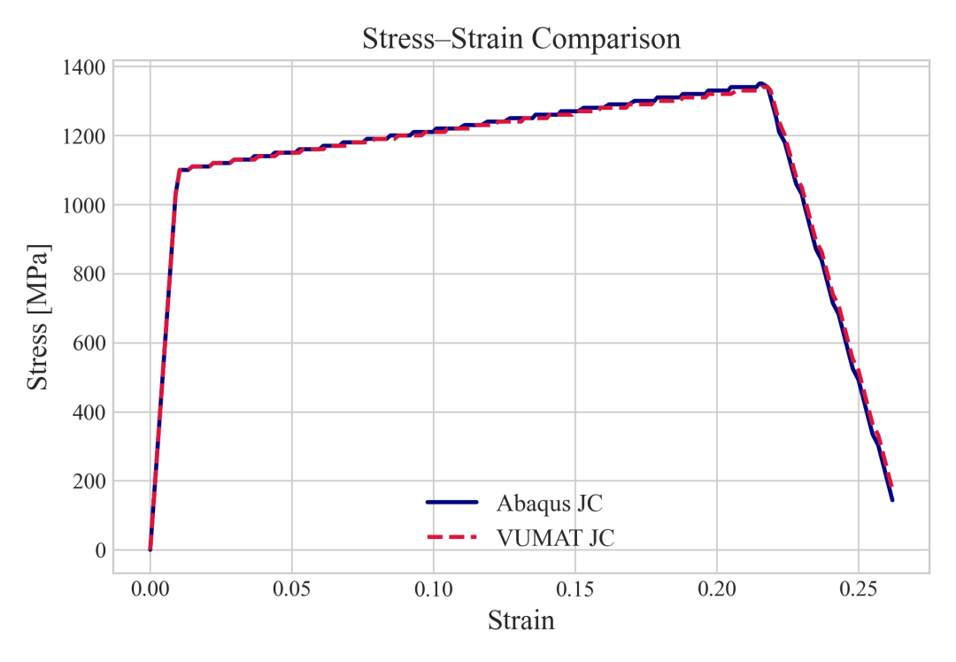
登录后免费查看全文
著作权归作者所有,欢迎分享,未经许可,不得转载
首次发布时间:2026-05-27
最近编辑:4月前

博士
签名征集中

还没有评论
相关推荐
最新文章
热门文章
