ANSYS Aqwa 用户手册15.0-(Aqwa Users Manual)

摘要:
本文为 ANSYS Aqwa 15.0 官方用户手册,基于 Workbench 平台,系统讲解海洋工程结构水动力仿真全流程。手册涵盖几何导入、部件属性定义、网格划分、连接与系泊、环境载荷施加、分析设置及结果后处理等核心模块,支持面 / 线体、点质量、浮心、阻尼、附加质量等模型配置。提供线性 / 非线性缆索、悬链线、护舷、铰接等连接方式,可模拟波浪、风、流载荷及缆索绞车、破断等工况。支持频域绕射与时域响应分析,输出 RAO、辐射阻尼、二阶力、张力、运动响应等结果,适用于船舶、海洋平台等结构评估,为工程仿真提供标准化操作指南。
Aqwa User's Manual
Copyright and Trademark Information
© 2013 SAS IP, Inc. All rights reserved. Unauthorized use, distribution or duplication is prohibited.
ANSYS, ANSYS Workbench, Ansoft, AUTODYN, EKM, Engineering Knowledge Manager, CFX, FLUENT, HFSS and any and all ANSYS, Inc. brand, product, service and feature names, logos and slogans are registered trademarks or trademarks of ANSYS, Inc. or its subsidiaries in the United States or other countries. ICEM CFD is a trademark used by ANSYS, Inc. under license. CFX is a trademark of Sony Corporation in Japan. All other brand, product, service and feature names or trademarks are the property of their respective owners.
Disclaimer Notice
THIS ANSYS SOFTWARE PRODUCT AND PROGRAM DOCUMENTATION INCLUDE TRADE SECRETS AND ARE CONFID- ENTIAL AND PROPRIETARY PRODUCTS OF ANSYS, INC., ITS SUBSIDIARIES, OR LICENSORS. The software products and documentation are furnished by ANSYS, Inc., its subsidiaries, or affiliates under a software license agreement that contains provisions concerning non-disclosure, copying, length and nature of use, compliance with exporting laws, warranties, disclaimers, limitations of liability, and remedies, and other provisions. The software products and documentation may be used, disclosed, transferred, or copied only in accordance with the terms and conditions of that software license agreement.
ANSYS, Inc. is certified to ISO 9001:2008.
U.S. Government Rights
For U.S. Government users, except as specifically granted by the ANSYS, Inc. software license agreement, the use, duplication, or disclosure by the United States Government is subject to restrictions stated in the ANSYS, Inc. software license agreement and FAR 12.212 (for non-DOD licenses).
Third-Party Software
See the legal information in the product help files for the complete Legal Notice for ANSYS proprietary software and third-party software. If you are unable to access the Legal Notice, please contact ANSYS, Inc.
Published in the U.S.A.
Chapter 1: Aqwa Introduction: What is Aqwa?
ANSYS Aqwa provides an engineering toolset for the investigation of the effects of wave, wind and
current on floating and fixed offshore and marine structures, including: spars; floating production,
storage, and offloading (FPSO) systems; semi-submersibles; tension leg platforms (TLPs); ships; renewable energy systems; and breakwater design.
Aqwa Hydrodynamic Diffraction provides an integrated environment for developing the primary hydro-
dynamic parameters required for undertaking complex motions and response an alyses. Three-dimen-
sional linear radiation and diffraction ana lysis may be undertaken with multiple bodies, taking full account of hydrodynamic interaction effects that occur between bodies. While primarily designed for floating
structures, fixed bodies such as breakwaters or gravity-based structures may be included in the models. Computation of the second-order wave forces via the full quadratic transfer function matrices permits use over a wide range of water depths.
Aqwa Hydrodynamic Diffraction can also generate pressure and inertial loading for use in a structural an alysis as part of the vessel hull design process. The results from a diffraction an alysis can be mapped onto an ANSYS Mechanical finite element model for further structural assess ment and detailed design. Since the mapping function automatically accounts for mesh differences between the hydrodynamic
and finite element models they do not have to be topologically identical.
Aqwa Hydrodynamic Time Response provides dynamic an alysis capabilities for undertaking global per- formance assess ment of floating structures in the time domain. A wide range of physical connections, such as mooring lines, fenders, and articulations, are provided to model the restraining conditions on
the vessels. In addition, sea-keeping simulation may be undertaken with the inclusion of forward speed effects. Slow-drift effects and extreme-wave conditions may be investigated, and damage conditions,
such as line breakage, may be included to study any transient effects that may occur.
Chapter 2: Aqwa Approach
This chapter takes you through the different steps required to setup a hydrodynamic an alysis.
2.1. Import or Create Hydrodynamic An alysis Systems
2.2. Attach Geometry
2.3. Define Parts Behavior
2.4. Define Connections
2.5. Mesh
2.6. Establish An alysis Settings
2.7. Applying Ocean Environment and Forces
2.8. Solution
2.1. Import or Create Hydrodynamic An alysis Systems
You can import an existing Aqwa Editor (v12.0) database into Workbench, or you can create a new hy- drodynamic system in the Workbench Project Schematic.
2.1.1. Import a Hydrodynamic System Database
2.1.2. Create a Hydrodynamic An alysis System
2.1.1. Import a Hydrodynamic System Database
To import an existing hydrodynamic system database, do the following:
1. In Workbench, click on the Import button (or select File>Import).
2. In the Import window, select Files of type: AQWAWB Database (大 .aqdb).
3. Click on a .aqdb database, and select Open to open the Aqwa Editor and create an Aqwa Hydrodynamic Diffraction system for each An alysis contained within the database.
The above technique may be used to duplicate complex connected systems that you cannot otherwise replicate using the Duplicate function. Once saved in Workbench as a Workbench project, you may use Workbench File>Open to open an existing Workbench Project containing hydrodynamic systems.
2.1.2. Create a Hydrodynamic An alysis System
Each ana lysis type is represented by an ana lysis system that includes the individual components of the ana lysis such as the associated geometry and model properties. Most a nalyses are represented by one independent an alysis system. However, an an alysis with data transfer can exist where results of one
a nalysis are used as the basis for another a nalysis. In this case, an ana lysis system is defined for each a nalysis type, where components of each system can share data.
• To create an ana lysis system, expand the Ana lysis Systems section in the Toolbox and drag an an alysis object template onto the Project Schematic. The ana lysis system is displayed as a vertical array of cells (schematic) where each cell represents a component of the a nalysis system. Address each cell by right- clicking on the cell and choosing an editing option.
• To create an an alysis system with data transfer to be added to an existing system, drag the object template representing the upstream a alysis directly onto the existing system such that red boxes enclose cells that will share data between the systems. After you release the mouse button, the two systems are dis- played, including an interconnecting link and a numerical designation as to which cells share data.
See Working through a System for more information.
Note
In hydrodynamic a nalysis systems, the Geometry cell is the only cell that can share data with other types of an alysis systems.
2.2. Attach Geometry
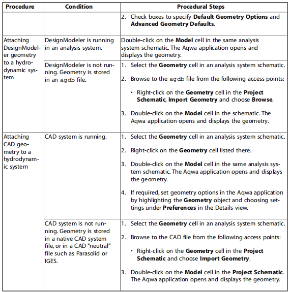
There are no geometry creation tools in the Aqwa application so geometry must be attached to the hydrodynamic system. You can create the geometry from either of the following sources:
• From within Workbench using DesignModeler. See the DesignModeler Help for details on the use of the various creation tools available.
• From a CAD system supported by Workbench. See the CAD Integration section for a complete list of the supported systems.
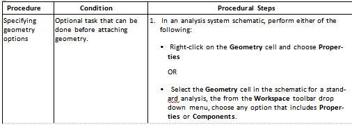
Before attaching the geometry from either of these sources, you can specify several options that de-
termine the characteristics of the geometry you choose to import by right clicking on the Geometry
cell and choosing Properties. See the CAD Integration section for more details about the options, most of which do not apply in hydrodynamic an alyses. Also see the General Modeling Requirements section for more information about the implications of Geometry import properties.
Note
Aqwa only processes the Line Bodies and Surface Bodies in a geometry. Make sure that the boxes are checked for both of these Geometry options in the Properties view. You can attach a geometry that has no line or surface bodies, but Aqwa will not process the geometry.
Related Procedures
CAD Interface Terminology
The CAD interfaces can be run in either plug-in mode or in reader mode.
• Attaching geometry in plug-in mode: requires that the CAD system be running.
• Attaching geometry in reader mode: does not require that the CAD system be running.
2.2.1. General Modeling Requirements
DesignModeler is the ANSYS tool used to create geometry for hydrodynamic systems. For information
on importing geometry created in DesignModeler, see the Geometry section. When using DesignModeler
to define the geometry there are a number of aspects that you should consider to ensure that your model is suitable for an alysis with Aqwa, such as:
• Ensure that the model is split at the water line, which must lie on the XY plane. Import or create each structure, use Translate operations to set the correct draft or depth for each structure, and then use
a Slice operation to split the surface bodies at water level.
• When using lines to create beams, only tubular sections are supported in Aqwa; all other sections
will result in a stub element being formed and you will need to define additional information in the Aqwa application. Lines should be created using Add Frozen Operation on the Line Details, and
consist of only 1 Point Segment per line.
• Each vessel / structure should be a part, so all the bodies that you have should be grouped via the multibody part facility. Note, it is not possible to rename these within the Aqwa application.
• The model is oriented with its Z axis vertical up.
• Surfaces must have normals pointing outward.
Hydrodynamic an alysis systems only process the Line Bodies and Surface Bodies in a geometry. By default, Line Bodies are not imported with the geometry. To change this default setting, in the Workbench
window, select Tools > Options and click on the Geometry Import entry in the tree. Make sure that the boxes are checked for Solid Bodies, Surface Bodies and Line Bodes as needed. You can attach a geometry that has no line or surface bodies, but this is not appropriate for an Aqwa an alysis.
You can also set the Geometry import options on a per system basis. When a system is initially created, the default geometry import settings will be used. If you would like to change the import settings for
a particular system, right click on the Geometry cell in that system and select Properties. Use the check boxes in the Properties view to set the items to import for this system. These settings are sent to the editor to use on edit or import. If you change the settings after initially editing the model you will need to refresh the cell, or edit and refresh, to consume the change and reattach the geometry with the new CAD import settings.
2.2.2. Configuring the Geometry
On opening a hydrodynamics an alysis system the Aqwa Editor will automatically attach the geometry. Each part becomes a separate structure in Aqwa. If a structure is to be formed of both diffracting and non-diffracting elements, these should be in separate defined bodies within the (multi-body) part.
When attaching a geometry, the units also change to be those of the model; these can be modified via the units menu if desired.
The hydrodynamics systems assume the still water surface lies on the XY plane, and Z is positive up.
All structures are located in a global an alysis space; note that Hydrostatic Results and Hydrodynamic Graphical Results are also presented in global directions.
Within the geometry you can select the types of bodies that will be attached.
Once attached the diffracting behavior of surface geometry can be selected; lines can be set to be Tu- bular (TUBE Elements) or Slender Tube (STUB elements) and additional Aqwa specific objects can be added, such as Point Mass, Point Buoyancy and Disc.
The Details panel provides you with options for setting up the sea geometry’s Water Depth and size
(Water Size X, Water Size Y), which can be used to alter the graphical view. By Slicing on the XY plane,
the sea level coincides with the point where the surface geometry is split to form above water (non- diffracting) and below water (diffracting) sections. By default, this setting in the Surface Body Details view will be Program Controlled and determined from the water level; however, you can manually
override it to define specific bodies to be non-diffracting.
It is important that the correct water depth is specified, especially with shallow water conditions, since the sea bed acts as a boundary condition to the diffraction a nalysis. The Water Size in the X and Y dir- ections modifies the extent of the graphical display of the water surface and sea bed.
The Water Density can also be changed.
Note
It is not yet possible to employ symmetry in the Aqwa Editor, hence the full model must be meshed.
2.2.3. Add Fixed Points
A Fixed Point is a non-moving point defined as part of your geometry. Fixed connection points are
defined in the Details panel by entering coordinates in global space or specifying an offset from a vertex on a structure. The coordinates defining the connection point can be parameterized. A fixed point does not move with any structure (even if it is initially defined as offset from a point on a structure). A fixed
point can be used by more than one object (cable, fender, etc.), if required. The option to choose a fixed point vs. connection points on structures is controlled by the Connectivity field in the Details panel of the object using the connection points.
To add a fixed point, click on the Geometry object in the tree, and from the Add menu in the toolbar or the right click menu, select Fixed Point. Click on the Fixed Point object that was added and do one of the following:
• Set Definition of Position to Coordinates, and set the Position Coordinates (X Ordinate, Y Ordinate, Z Ordinate) in the Details panel.
• Set Definition of Position to Vertex Selection. Click on Select a Single Vertex in the Vertex field, select a vertex on a structure, and click Apply. You can then set an X Offset, Y Offset, or Z Offset from the
vertex if needed.
Note
It is assumed that fixed points are on the sea bed for catenary cables. Prior to Release 15.0, these objects were labeled as “Connection Point”.
2.3. Define Parts Behavior
A part is a group of geometric entities that form a ship or other structure that is to be an alyzed in Aqwa. The name is read in from the geometry database and the graphical view will show the part; the appro- priate structure will be highlighted when the part in the tree is selected. Each part will be assigned a
structure number for the an alysis. The parts can be included or excluded from the an alysis using the Structure Selection.
A number of options can be set for each part in the Details panel.
To help visualization, it is possible to show or hide specific parts using the Part Visibility option. The Part Activity option is used to decide what structures are used in the an alysis.
Note
If a part is suppressed, it cannot be used in the an alysis. However, when a part is unsup- pressed, it must be added to the Structure Selection in order for it to be included in the an alysis.
Total Structural Mass, and X, Y, and Z Positions of COG (the Center of Gravity) are displayed for each Part. This information is based on the masses defined for each element/body of the structure: Point
Masses and Tubes/Stubs. It is important to remember that the mass of each Point Mass is defined either manually by the user, or automatically by the program after the hydrostatic calculation has been done and is up-to-date. If the hydrodynamic diffraction system is not up to date, this information is solely
based on the initial 1kg mass attributed to each point mass, if its definition is Program Controlled, or on any subsequent out-of-date hydrostatic an alysis.
If an internal lid is required to prevent irregular frequency problems then Generate Internal Lid can
be set to Yes and it will be automatically generated during the Aqwa an alysis. Note that an automatically generated lid will not be displayed. Alternatively, a manually generated lid may be used; create an ap-
propriate plane surface as a Surface Body; set Structure Type to Abstract Geometry and Abstract Type to Internal Lid. If you have a structure with a moon pool where large resonant waves may occur, then
you can form an external lid using a predefined geometry Surface Body with Structure Type set to Abstract Geometry and Abstract Type to External Lid.
The Current Calculation Depth defines the depth below the water surface at which the current velocity is to be computed for use in the calculation of the hull drag loading. By default the current at the water surface is used. Note that hull drag loads are only included if Current Force Coefficients are defined for
the part.
By default the structure is set to be free to move. Alternatively, the whole structure can be fixed by
setting Structure Fixity to Structure is Fixed in Place. Fixity primarily affects the results of a hydrodynamic diffraction ana lysis by impacting the structure's RAOs. It therefore also has an impact on the hydrodynamic time response results as the calculated drift forces depend on these RAOs. It is thus necessary to impose the coherence between the setup of the two an alyses by fixing the structure in the time response
an alysis. Since the user can create joints to be used in time response an alysis, it is the user's responsib-
ility to create a rigid joint when it is connected to a fixed point on any Part marked as Fixed in the Details dialog. Not doing so will result in an error when solving the time response an alysis.
The Mass Factor and Drag Factor provide a way of modifying the added mass and drag coefficients defined for any tube and disc elements associated with this part. This may be used for parametric
studies where the effects of Morison drag on appropriate elements are considered important (e.g. sim- ulating tests at model scale). These factors have no effect on any other object type in the part.
The Slam Factor provides a way to enable the computation of slamming loads on tube and disc elements. By default a factor of zero is specified which disables this computation. Any positive non-zero value
will cause the program to compute the slam coefficient for each applicable element, based on the
premise that the slam force is equal to the rate of change of the added mass tensor (with time) multiplied by the velocity. The resulting coefficient is then multiplied by this factor. This may be used for parametric studies where the effects of slamming loads on tube and disc elements are considered important (e.g.
simulating tests at model scale). This factor has no effect on any other object type in the part.
Slamming loads can also be included for stub elements by setting the Slam Factor to a positive non-
zero value, but the magnitude of the factor is immaterial in this case because a value of unity is always employed in the an alysis.
Note
The method for computing the slam coefficient requires that the time-step used in a time
history an alysis must be sufficiently s mall to accurately represent the added mass at each
stage of immersion/emergence. In general this will depend on the geometry of each element and its orientation to the water surface. In practice, this severe restriction of the size of the
time-step means that this facility is only used when specifically investigating the effects of slam forces on individual elements during critical stages of the simulation period, as the
momentum change due to slam forces are normally s mall and have little effect on the overall motion of the structure.
Submerged Structure Detection is Program Controlled by default, and Aqwa will detect the highest point (greatest Z coordinate) and check whether it is below the water level; alternatively this automatic detection can be overridden.
The Metacentric Heights can be overridden about both the global X (Override Calculated GMX = Yes) or Y (Override Calculated GMY = Yes) axes to modify the hydrostatic stiffness of the vessel. When
these are overridden, Aqwa first calculates the hydrostatic stiffness matrix based only on the cut water
plane and displaced volume properties. It then adjusts the second moments of area IXX, IYY and recal- culates its associated properties, PHI (principal axis), GMX/GMY, BMX/BMY etc. to give the required GM
values. The associated additional hydrostatic stiffness is calculated automatically and stored in the hy-
drodynamic database. If the GM value input is less than that based on the geometry alone, the resulting additional stiffness will be negative. This would be the case if ballast tanks were being modelled, making the structure less stable, statically.
Nonlinear roll damping moment can be calculated in slow drift time history an alyses to take into account the effect of vortex shedding from the bilges of a vessel. The method is based on "An Engineering As-
sess ment of the Role of Non-linearities in Transportation Barge Roll Response", Robinson and Stoddart, Trans. R.I.N.A 1986.
Whether vortex shedding is occurring or not is calculated by the program based on the relative flow velocity at the bilge, Keulegan-Carpenter number, roll natural frequency of the vessel, and the radius of the bilge. The roll damping coefficient used in the nonlinear roll damping force calculation is also calculated by the program based on a database stored within the program.
To compute the effects of nonlinear roll damping, select Included in Calculations from the Non-Linear
Roll Damping drop down menu. By default these are excluded from the calculations. If selected, addi-
tional parameters need to be provided. It is assumed that the two bilges have symmetric properties
about the center line of the vessel. The Bilge Radius defines the local radius of the bilge corner (dimen- sion from the hull to the extreme of the bilge). The Depth to Bilge is the vertical position of the bilge
corner on the vessel in the global axis system. The Offset of Bilge from Central Line is the lateral offset of the bilge corner from the center line of the vessel in the global axis system. The central line is defined by selecting vertices from the geometry for the start and end points of the central line (Reference
Vertex for Start of Central Line, Reference Vertex for End of Central Line). For each end of the central line, you can also specify X and Y offsets.
Note
The vertical position of the vertices selected for the central line end points is irrelevant; the vertical position of the central line is set by Depth to Bilge.
Additional Hydrodynamic Stiffness, Damping and Added Mass can be added to the Part object using the context menu, or from the Add menu on the toolbar when the Part is selected.
Use the context (right click) menu or the toolbars to add additional Aqwa specific elements into the geometry, such as: Point Mass, Point Buoyancy, Disc, Wind Force Coefficients, and Current Force Coeffi- cients. You can remove any of the objects by right clicking on them in the tree and selecting Delete from the context menu.
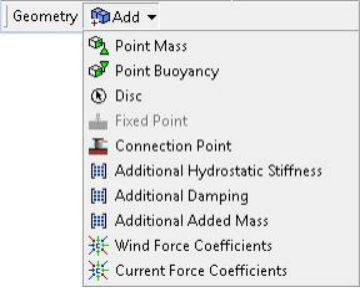
A full list of the types of bodies is:
2.3.1. Surface Body
2.3.2. Line Body
2.3.3. Point Mass
2.3.4. Point Buoyancy
2.3.5. Disc
2.3.6. Additional Hydrodynamic Stiffness
2.3.7. Additional Damping (Frequency Independent)
2.3.8. Additional Added Mass (Frequency Independent)
2.3.9. Current Force Coefficients
2.3.10. Wind Force Coefficients
2.3.11. Structure Connection Points
2.3.1. Surface Body
Surface bodies are areas that can be meshed to create diffracting or non-diffracting elements for the Aqwa an alysis. The name of the surface body will be obtained from that given in Design Modeler and it cannot be changed here.
If a body is not required for the an alysis it can be suppressed (Body Activity). Suppressed bodies will not be meshed and will be excluded from the an alysis. You can hide the body in the graphic window (Body Visibility), in which case it will not be shown but will be included in the a nalysis.
It is possible to change the type of surface from a Physical Geometry to an Abstract Geometry (Structure Type). For physical geometry, Program Controlled Surface Type will set all surface bodies below the
water surface as diffracting and those above will be non-diffracting. If required, those below the water surface can be manually defined as non-diffracting elements for the an alysis. This may be required, for instance, when part of the structure is in contact with the sea bed, or where contact occurs underwater between adjacent parts.
For an abstract geometry, Abstract Type provides a number of options to select how this geometry is
to be used. If an area is of particular interest, then the Custom Results Positions option enables a mesh to be applied and each node of the mesh will form a field point element; additional information will
be available at these points. Alternatively, Internal Lid and External Lid can be used to suppress standing waves either between structures or within structures.
Note
Automatic internal lids can be selected using the Part option.
If the generation of an external lid is specified, two additional parameters are required. The first is a Lid Damping Factor, set between 0 and 1. The factor represents how effective the lid is to be; 0 will result in no effect, while 1 will prevent any vertical water surface velocity under the lid.
The second parameter is the Gap for Lid. It is a representative size for the lid; typically the distance
between the two vessels or the width of a moon-pool. It enables the lid properties to be tuned to the resonant frequency of waves in the gap.
2.3.2. Line Body
Line bodies are used to create single elements for Aqwa. How they are interpreted depends upon the cross section of the line; if it has a circular cross section, then it will be automatically converted into a
tubular line and will create standard tubular (TUBE) elements. All other sections will create slender tube (STUB) elements. The content of the details pane changes considerably depending upon the type of
line. The details are discussed below.
Line type: Tubular
If the line in Design Modeler was defined with a tubular section, the line body will default to this setting; the tube Diameter and Thickness are automatically read from the Design Modeler data, along with the calculated inertia values.
Use Tube Type to make the tube Sealed or Floodable. By default, the tube is sealed, and in this case
the tube would be buoyant; however, the tube does not have longitudinal drag or added mass unless
discs are created at the ends. Discs can automatically be applied at either (Created at End A Only, Created at End B Only) or both (Created at Both Ends) ends with the Tube End Discs option; if you choose one
of these options, default disc parameters are used. If you require different parameters, discs can be ex- cluded here and added manually.
A Viscous Drag Coefficient and Added Mass Coefficient can be defined, although drag is not used in Hydrodynamic Diffraction or hydrostatic an alyses. A density of the tube (Material Density) is also required; this defaults to the standard value for steel.
Line type: Stub
For all sections other than tubular, only the inertias will be obtained automatically from the parameters that are entered in Design Modeler. If a stub element is not required, then it is possible to change it to a tubular line and define the diameter and thickness within the Aqwa Editor.
There are options to change the diameter of a stub element in both the local Z and Y directions (Z
Diameter, Y Diameter), as well as the Cross Section Area. For Aqwa, valid cross sectional areas vary between an ellipse and a rectangle with the width and height of the two diameters. In addition, you can specify a Viscous Drag Coefficient and Added Mass Coefficient in each of the Z and Y directions. It is also possible to define the mass contribution of the stub to the model (Mass/Unit Length). You
cannot automatically add Discs to STUB objects, but you can add them manually if needed.
2.3.3. Point Mass
Point mass elements can be inserted into the model; the properties can either be input manually or can be Program Controlled.
If Mass definition is set to Manual, the point mass must have all its properties input by the user (Mass, X, Y, and Z coordinates). If a Program Controlled point mass is used, the mass and the horizontal position will be calculated from the panel elements in the structure (i.e. excluding tubular stub lines and point
buoyancy bodies). The mass will equal the mass of water displaced, and the horizontal position will be that of the center of buoyancy.
The moments of inertia (or radii of gyration) and vertical position (Z) cannot be determined by the
program and must always be input. Moments of inertia can be defined directly or by inputting radii of gyration. If Define inertia values by is set to via Radius of Gyration, you need to enter Kxx, Kyy, and Kzz. If you select Direct input of Inertia, you must enter the Ixx, Iyy, and Izz values.
Tip
After inserting your point masses, solve for hydrostatics only; then the hydrostatic results will be available and the values of mass will be calculated before performing the full Aqwa a nalysis.
2.3.4. Point Buoyancy
Point buoyancy (PBOY) elements can be inserted into the model; these require a position (X, Y, Z) and a Volume.
2.3.5. Disc
Disc elements can be used to create an area that has drag (Viscous Drag Coef) and added mass (Added Mass Coef) in the direction perpendicular to the disc. The Diameter of the disc is required along with
the centroid and the definition of the normal direction. If the centroid is at the position of an existing vertex, set Centroid Definition to Select Vertex and click Pick in the Vertex field; then select the vertex on the model and click Apply. To enter the coordinates of the vertex directly, set Centroid Definition to Specify Coordinates, and enter the X, Y, and Z values.
You can specify the normal by picking a second vertex or specifying the direction of a normal vector.
To use an existing vertex to define the normal, set Normal Definition to Select Second Vertex and click on Pick in the Normal Vertex field; then select the vertex on the model and click Apply. To enter the vector for the normal directly, set Normal Definition to Specify Vector Components, and enter the Normal X, Normal Y, and Normal Z component values.
The default values of the added mass and viscous drag coefficients can be modified if desired.
Note
Drag is not used in hydrodynamic diffraction an alyses.
2.3.6. Additional Hydrodynamic Stiffness
This object may be used to input an additional linear hydrostatic stiffness matrix using tabular input in the Matrix Definition Data window. The linear stiffness matrix relates to the hydrostatic forces contrib- uting to the equations of static equilibrium of a structure. Specifically, the net linear hydrostatic forces F(s), acting at the center of gravity of a structure, when the structure is at an arbitrary position X, are
given by:
F(s) = (K + dK) ( X(e) - X ) + B(e)
• K = stiffness matrix
• dK = additional hydrodynamic stiffness matrix input in this object
• X(e) = equilibrium position
• B(e) = buoyancy force at equilibrium
If additional hydrodynamic stiffness is used it should be checked that the above expression, which is used to calculate the linear hydrostatic forces throughout the Aqwa suite, produces the forces on the structure intended by the user.
Note
In this context, hydrostatic forces can act in all 6 degrees of freedom.
In the equation above, the term X(e) is the diffraction an alysis defined position. If the initial position in a subsequent motions ana lysis is not as defined in the diffraction run, then there will be restoring forces which will try to return the structure to the diffraction defined position.
To add an Additional Hydrodynamic Stiffness Matrix:
1. Select a part in the Tree Outline.
2. Right click on the part and select Add > Additional Hydrodynamic Stiffness.
or
Click on the Add icon in the toolbar and select Additional Hydrodynamic Stiffness from the dropdown list.
An Additional Hydrodynamic Stiffness object is added to the part.
3. Select the Additional Hydrodynamic Stiffness object in the Tree Outline and enter the matrix coefficients in the Matrix Definition Data window that appears below the model.
2.3.7. Additional Damping (Frequency Independent)
This object may be used to input frequency independent additional damping in global directions using tabular input. Only one definition of Additional Damping per structure can be active (i.e. not suppressed) for the ana lysis and the values are added to those calculated automatically during the an alysis.
To add Additional Damping:
1. Select a part in the Tree Outline.
2. Right click on the part and select Add > Additional Damping.
or
Click on the Add icon in the toolbar and select Additional Damping from the dropdown list.
An Additional Damping object is added to the part.
3. Select the Additional Damping object in the Tree Outline and enter the matrix coefficients in the Matrix Definition Data window that appears below the model.
2.3.8. Additional Added Mass (Frequency Independent)
This object may be used to input frequency independent additional added mass in global directions using tabular input. Only one definition of Additional Added Mass per structure can be active (i.e. not suppressed) for the an alysis and the values are added to those calculated automatically during the
an alysis.
To add Additional Added Mass:
1. Select a part in the Tree Outline.
2. Right click on the part and select Add > Additional Added Mass.
or
Click on the Add icon in the toolbar and select Additional Added Mass from the dropdown list.
An Additional Added Mass object is added to the part.
3. Select the Additional Added Mass object in the Tree Outline and enter the matrix coefficients in the Matrix Definition Data window that appears below the model.
2.3.9. Current Force Coefficients
This object may be used to include the viscous drag of the current on the hull of a fixed or floating
structure, using tabular input in the Current Force Coefficients window. The term current force coefficient is used to differentiate these coefficients from traditional drag coefficients and from coefficients of wind force.
The current force coefficients are defined as the force or moment per unit velocity squared. The moment is about the center of gravity of the structure. These forces are a function of the relative velocity between
the structure and the water. This means that the current coefficient should still be input even when there is no current present, as the relative velocity is generally non-zero for a dynamic ana lysis.
To add a Current Force Coefficients object:
1. Select a part in the Tree Outline.
2. Right click on the part and select Add > Current Force Coefficients.
or
Click on the Add icon in the toolbar and select Current Force Coefficients from the dropdown list.
A Current Force Coefficients object is added to the part.
3. Select the Current Force Coefficients object in the Tree Outline and enter the coefficients in the Coefficient Data window that appears below the model. Enter the Direction of the current (-180 to +180 degrees),
the X force coefficient (Translation X), Y force coefficient (Translation Y), Z force coefficient (Translation Z), Rotation about X coefficient (Rotation X), Rotation about Y coefficient (Rotation Y), and Rotation
about Z coefficient (Rotation Z). The number of rows is increased as each entry is made, up to a maximum of 41 rows.
Note that the forces are in the directions of the axes, not in the direction of the current. For example, for relative current velocity V in direction φ:
force in X direction = CUFXφ.V2
force in Y direction = CUFYφ.V2
moment about Z axis = CURZφ.V2
where CUFX, CUFY and CURZ are the coefficients. Similar equations apply for force in Z and moments about X and Y.
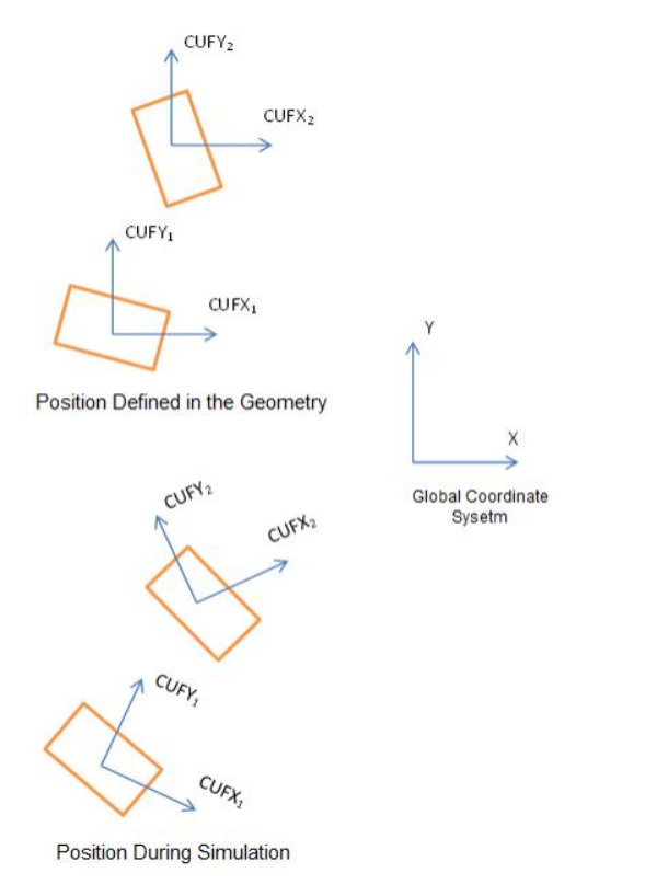
The coefficients are applied in a moving axis system; in other words, the axes move with the structure.
Since there is no structure local axis system available, the initial coefficient data must be defined relative
to the global coordinate system when the structure is in the position as defined in the geometry. For example:
Note
• You may have multiple Current Force Coefficient objects in the an alysis, but only one can be enabled during an ana lysis (an error will be reported when solving if multiple objects are en- abled).
• There is a limit of 41 unique directions for the enabled Wind Force Coefficient and Current
Force Coefficient tables combined. Each table may have an entry for the same Direction value.
• If a direction is specified for Wind Force Coefficients that does not exist for Current Force
Coefficients then linearly interpolated values will be utilized for the Current Force Coefficients for that direction, based upon adjacent defined directions.
• An error will be reported if there are multiple entries having the same value of Direction in the table.
详细内容请见附件
免责声明:
本页面/内容部分素材来源于互联网公 开 信 息,旨在传递更多信息,不代表本平台立场。
版权归原作者或机构所有,如涉及侵权,请通过平台联系我们,我们将在核实后第一时间处理。
本平台对转载内容的真实性、准确性不作任何保证,用户需自行判断并承担使用风险。