嵌入式实时操作系统：DSP 微内核设计与实现电子书 212页

4月前浏览740

嵌入式实时操作系统：DSP 微内核设计与实现（DSP_Realtime_Operating_Systems_for_Embedded_Systems）电子书

摘要：

本书是嵌入式 DSP 实时操作系统微内核设计与实现的专业指南，围绕嵌入式实时操作系统内核开发展开系统讲解。先明确嵌入式系统对内存、性能、可移植性的核心需求，再阐述抢占式多任务、任务控制块、信号量、环形缓冲队列等核心概念与原理。书中完整呈现内核架构、硬件适配、任务切换、中断处理、进程通信、串口 I/O、内存管理的代码实现，覆盖系统启动、任务创建 / 调度 / 销毁全流程，提供基于 MC68000 系列处理器的工程实例与调试监控工具，还详解跨平台开发环境搭建与移植方法，为嵌入式 DSP 实时内核开发提供全栈技术参考。

Realtime Operating Systems

Concepts and Implementation of Microkernels for Embedded Systems

Dr. Jürgen Sauermann, Melanie Thelen

Preface

Every year, millions of microprocessor and microcontroller chips are sold as CPUs for general purpose computers, such as PCs or workstations, but also for devices that are not primarily used as computers, such as printers, TV sets, SCSI controllers, cameras, and even coffee machines. Such devices are commonly called embedded systems. Surprisingly, the number of chips used for embedded systems exceeds by far the number of chips used for general purpose computers.

Both general purpose computers and embedded systems (except for the very simple ones) require an operating system. Most general purpose computers (except mainframes) use either UNIX, Windows, or DOS. For these operating systems, literature abounds. In contrast, literature on operating systems of embedded systems is scarce, although many different operating systems for embedded systems are available. One reason for this great variety of operating systems might be that writing an operating system is quite a challenge for a system designer. But what is more, individually designed systems can be extended in exactly the way required, and the developer does not depend on a commercial microkernel and its ﬂaws.

The microkernel presented in this book may not be any better than others, but at least you will get to know how it works and how you can modify it. Apart from that, this microkernel has been used in practice, so it has reached a certain level of maturity and stability. You will learn about the basic ideas behind this microkernel, and you are provided with the complete source code that you can use for your own extensions.

The work on this microkernel was started in summer 1995 to study the efﬁciency of an embedded system that was mainly implemented in C++. Sometimes C++ is said to be less efﬁcient than C and thus less suitable for embedded systems. This may be true when using a particular C++ compiler or programming style, but has not been conﬁrmed by the experiences with the microkernel provided in this book. In 1995, there was no hardware platform available to the author on which the microkernel could be tested. So instead, the microkernel was executed on a simulated MC68020 processor. This simulation turned out to be more useful for the development than real hardware, since it provided more information about the execution proﬁle of the code than hardware could have done. By mere coincidence, the author joined a project dealing with automated testing of telecommunication systems. In that project, originally a V25 microcontroller had been used, running a cooperative multitasking operating system. At that time, the system had already reached its limits, and the operating system had shown some serious ﬂaws. It became apparent that at least the operating system called for major redesign, and chances were good that the performance of the microcontroller would be the next bottleneck. These problems had already caused serious project delay, and the most promising solution was to replace the old operating system by the new microkernel, and to design a new hardware based on a MC68020 processor. The new hardware was ready in summer 1996, and the port from the simulation to the real hardware took less than three days. In the two months that followed, the applications were ported from the old operating system to the new microkernel. This port brought along a dramatic simpliﬁcation of the application as well as a corresponding reduction in source code size. This reduction was possible because serial I/O and interprocess communication were now provided by the microkernel rather than being part of the applications.

Although the microkernel was not designed with any particular application in mind, it perfectly met the requirements of the project. This is neither by accident nor by particular ingenuity of the author. It is mainly due to a good example: the MIRAGE operating system written by William Dowling of Sahara Software Ltd. about twenty years ago. That operating system was entirely written in assembler and famous for its real-time performance. Many concepts of the microkernel presented in this book have been adopted from the MIRAGE operating system.

1 Requirements

1.1 General Requirements

Proper software design starts with an alyzing the requirements that have to be fulﬁlled by the design. For embedded systems, the requirements are deﬁned by the purpose of the system. General deﬁnitions of the requirements are not possible: for example, the requirements of a printer will deﬁnitely be different from those of a mobile phone. There are, however, a few common requirements for embedded systems which are described in the following sections.

1.2 Memory Requirements

The ﬁrst PCs ofthe early eighties had 40 kilobytes ofROM, 256 or 512 kilobytes of RAM, and optionally a hard disk drive with 5 or 10 megabytes capacity. In the mid-nineties, an off-the-shelf PC had slightly more ROM, 32 megabytes of RAM, and a hard disk drive of 2 or 4 gigabytes capacity. Floppy disks with 360 or 720 kilobyte capacity, which were the standard medium for software packages and backups, had been replaced by CD-ROM and tape streamers with capacities well above 500 megabytes. Obviously, capacity has doubled about every two years, and there is no indication that this trend will change. So why bother about memory requirements?

A PC is an open system that can be extended both in terms of memory and peripherals. For a short while, a PC can be kept up to date with technological developments by adding more memory and peripherals until it is ultimately outdated. Anyway, a PC could live for decades; but its actual lifetime is often determined by the increasing memory demands of operating systems and applications rather than by the lifetime of its hardware. So to extend the lifetime of a PC as much as possible and thus to reduce the costs, its conﬁguration has to be planned thoroughly.

For a given embedded system, in contrast, the memory requirements are known in advance; so costs can be saved by using only as much memory as required. Unlike PCs, where the ROM is only used for booting the system, ROM size plays a major role for the memory requirements of embedded systems, because in embedded systems, the ROM is used as program memory. For the ROM, various types of memory are available, and their prices differ dramatically: EEPROMs are most expensive, followed by static RAMs, EPROMs, dynamic RAMs, hard disks,

ﬂoppy disks, CD-ROMs, and tapes. The most economical solution for embedded systems is to combine hard disks (which provide non-volatility) and dynamic RAMs (which provide fast access times).

Generally, the memory technology used for an embedded system is determined by the actual application: For example, for a laser printer, the RAM will be dynamic, and the program memory will be either EEPROM, EPROM, or RAM loaded from a hard disk. For a mobile phone, EEPROMs and static RAMs will rather be used.

One technology which is particularly interesting for embedded systems is on-chip memory. Comparatively large on-chip ROMs have been available for years, but their lack of ﬂexibility limited their use to systems produced in large quantities. The next generation of microcontrollers were on-chip EPROMs, which were suitable also for s maller quantities. Recent microcontrollers provide on-chip EEPROM and static RAM. The Motorola 68HC9xx series, for example, offers on-chip EEPROM of 32 to 100 kilobytes and static RAM of 1 to 4 kilobytes.

With the comeback of the Z80 microprocessor, another interesting solution has become available. Although it is over two decades old, this chip seems to outperform its successors. The structure of the Z80 is so simple that it can be integrated in FPGAs (Field Programmable Logic Arrays). With this technique, entire microcontrollers can be designed to ﬁt on one chip, providing exactly the functions required by an application. Like several other microcontrollers, the Z80 provides a total memory space of 64 kilobytes.

Although the memory size provided on chips will probably increase in the future, the capacities available today suggest that an operating system for embedded system should be less than 32 kilobytes in size, leaving enough space for the application.

1.3 Performance

The increase in the PCs’ memory size is accompanied by a similar increase in performance. The ﬁrst PCs had an 8 bit 8088 CPU running at 8 MHz, while today a 32 bit CPU running at 200 MHz is recommended. So CPU performance has doubled about every two years, too. Surprisingly, this dramatic increase in performance is not perceived by the user: today’s operating systems consume even more memory and CPU performance than technological development can provide. So the more advanced the operating system, the slower the applications. One reason for the decreasing performance of applications and also of big operating systems might be that re-use of code has become common practice; coding as such is avoided as much as possible. And since more and more code is

executed in interfaces between existing modules, rather than used for the actual problem, performance steadily deteriorates.

Typically, performance demands of embedded systems are higher than those of general purpose computers. Of course, if a PC or embedded system is too slow, you could use a faster CPU. This is a good option for PCs, where CPU costs are only a minor part of the total costs. For embedded systems, however, the cost increase would be enormous. So the performance of the operating system has signiﬁcant impact on the costs of embedded systems, especially for single-chip systems.

For example, assume an embedded system requiring serial communication at a speed of 38,400 Baud. In 1991, a manufacturer of operating systems located in Redmond, WA, writes in his C/C++ Version 7.0 run-time library reference: “The _bios_serialcom routine may not be able to establish reliable communications at baud rates in excess of 1,200 Baud (_COM_ 1200) due to the overhead associated with servicing computer interrupts”. Although this statement assumes a slow 8 bit PC running at 8 MHz, no PC would have been able to deal with 38,400 baud at that time. In contrast, embedded systems had been able to manage that speed already a decade earlier: using 8 bit CPUs at even lower clock frequencies than the PCs’.

Performance is not only determined by the operating system, but also by power consumption. Power consumption becomes particularly important if an embedded system is operated from a battery, for example a mobile phone. For today’s commonly used CMOS semiconductor technology, the static power required is virtually zero, and the power actually consumed by a circuit is proportional to the frequency at which the circuit is operated. So if the performance of the operating system is poor, the CPU needs to be operated at higher frequencies, thus consuming more power. Consequently, the system needs larger batteries, or the time the system can be operated with a single battery charge is reduced. For mobile phones, where a weight of 140g including batteries and stand-by times of 80 hours are state ofthe art, both of these consequences would be show stoppers for the product. Also for other devices, power consumption is critical; and last, but not least, power consumption should be considered carefully for any electrical device for the sake of our environment.

1.4 Portability

As time goes by, the demands on products are steadily increasing. A disk controller that was the fastest on the market yesterday will be slow tomorrow. Mainstream CPUs have a much wider performance range than the different microcontroller families available on the market. Thus eventually it will be necessary to change to a different family. At this point, commercial microkernels can be a problem if they support only a limited number of microcontrollers, or not the one that would otherwise perfectly meet the speciﬁc requirements for a product. In any case, portability should be considered from the outset.

The obvious approach for achieving portability is to use high level languages, in particular C or C++. In principle, portability for embedded system is easier to achieve than for general purpose computers. The reason is that complex applications for general purpose computers not only depend on the CPU used, but also on the underlying operating system, the window system used, and the conﬁguration of the system.

A very s mall part of the microkernel presented in this book was written in Assembler; the rest was written in C++. The part of the kernel which depends on the CPU type and which needs to be ported when a different CPU family is used, is the Assembler part and consists of about 200 Assembler instructions. An experienced programmer, familiar with both the microkernel and the target CPU, will be able to port it in less than a week.

The entire kernel, plus a simple application, ﬁt in less than 16 kilobyte ROM for a MC68020 CPU. Hence it is especially suitable for single chip solutions.

2 Concepts

2.1 Speciﬁcation and Execution of Programs

The following sections describe the structure of a program, how a program is prepared for execution, and how the actual execution of the program works.

2.1.1 Compiling and Linking

Let us start with a variant of the well known “Hello World!” program:

#include <stdio.h>

const char * Text = "Hello World\n";

char Data [] = "Hello Data\n";

int Uninitialized; // Bad Practice

int main(int argc, char * argv [])

{

printf(Text);

}

This C++ program prints “Hello World”, followed by a line feed on the screen of a computer when it is executed. Before it can be executed, however, it has to be transformed into a format that is executable by the computer. This transformation is done in two steps: compilation and linking.

The ﬁrst step, compilation, is performed by a program called compiler. The compiler takes the program text shown above from one ﬁle, for example Hello.cc, and produces another ﬁle, for example Hello.o. The command to compile a ﬁle is typically something like

g++ -o Hello.o Hello.cc

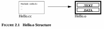
The name of the C++ compiler, g++ in our case, may vary from computer to computer. The Hello.o ﬁle, also referred to as objectﬁle, mainly consists of three sections: TEXT, DATA, and BSS. The so-called include ﬁle stdio.h is simply copied into Hello.cc in an early execution phase of the compiler, known as

preprocessing. The purpose of stdio.h is to tell the compiler that printf is not a spelling mistake, but the name of a function that is deﬁned elsewhere. We can imagine the generation of Hello.o as shown in Figure 2.1.1

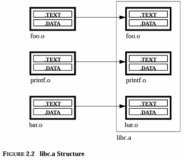
Several object ﬁles can be collected in one single ﬁle, a so-called library. An important library is libc.a (the name may vary with the operating system used): it contains the code for the printf function used in our example, and also for other functions. We can imagine the generation of libc.a as shown in Figure 2.2.

1. Note: The BSS section contains space for symbols that uninitialized when starting the program. For example, the integer variable Uninitialized will be included here in order to speed up the loading of the program. However, this is bad programming practice, and the bad style is not weighed up by the gain in speed. Apart from that, the memory of embedded systems is rather s mall, and thus loading does not take long anyway. Moreover, we will initialize the complete data memory for security reasons; so eventually, there is no speed advantage at all. Therefore, we assume that the BSS section is always empty, which is why it is not shown in Figure 2.1, and why it will not be considered further on.

The second step of transforming program text into an executable program is linking. A typical link command is e.g.

ld -o Hello Hello.o

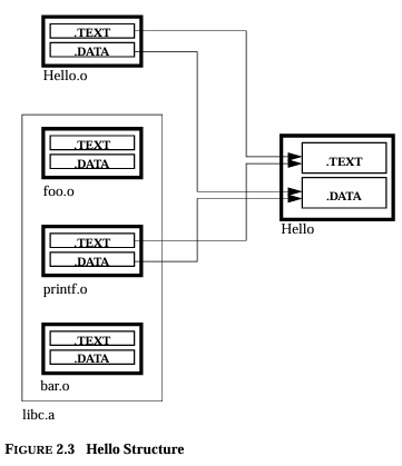
With the linking process, which is illustrated in Figure 2.3, all unresolved references are resolved. In our example, printfis such an unresolved reference, as it is used in main(), but deﬁned in printf.o, which in turn is contained in libc.a. The linking process combines the TEXT and DATA sections of different object ﬁles in one single object ﬁle, consisting of one TEXT and one DTA section only. If an object ﬁle is linked against a library, only those object ﬁles containing deﬁnitions for unresolved symbols are used. It should be noted that a linker can produce different ﬁle formats. For our purposes, the so-called Motorola S-record format will be used.

2.2 Loading and Execution of Programs

After a program has been compiled and linked, it can be executed. While compilation and linking is basically identical for embedded systems and general purpose computers, there are some differences regarding the execution of programs. Table 2.1 lists the steps performed during program execution and shows the differences between general purpose computers and embedded systems:

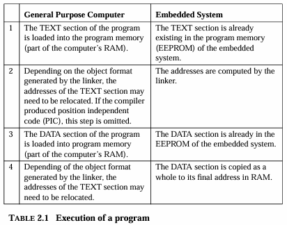
Obviously, the execution of a program in an embedded system is much easier than in a general purpose computer.

更多内容见附件

免责声明：

本页面/内容部分素材来源于互联网公开信息，旨在传递更多信息，不代表本平台立场。

版权归原作者或机构所有，如涉及侵权，请通过平台联系我们，我们将在核实后第一时间处理。

本平台对转载内容的真实性、准确性不作任何保证，用户需自行判断并承担使用风险。

Maxwell在电机设计与验证的计算案例-以永磁电机为例

摘要：本文为ANSYSMaxwell17.0版本永磁同步电机（PMSM）设计与验证案例，依托RMxprt与Maxwell联合完成全流程分析。先在RMxprt搭建6极36槽、额定功率20kW、转速1000rpm的电机模型，仿真得满载效率74.47%等关键参数；再一键生成Maxwell2D与3D瞬态模型，完成边界、激励、网格与求解设置，2D改用外部电路激励，3D直接施加电压激励并简化设置以提速。仿真结果显示，2D输出功率19.1kW，3D为18.1kW，与RMxprt吻合；2D与3D损耗差异源于端部绕组影响，整体验证了联合仿真方法的可靠性。Workshop5.1:PMSMExampleIntroductiontoANSYSMaxwellOverview•PMSMExample–ThisworkshopwilldiscusshowtouseRMxprtinconnectiontoMaxwellinordertodevelopacompleteanalysisofaPMSM(PermanentMagnetSynchronousMachine).–Thefollowingtaskswillbeperformed:•CreatetheRMxprtmodel•RMxprtResultsAnalysis•CreatetheMaxwell2DModelfromRMxprt•Analyzethemodel•Review/Post-processMaxwell2Dresults•CreatetheMaxwell3DModelfromRMxprt•Analyzethemodelandmodifyexcitationstosavesimulationtime•AnalyzeMaxwell3DresultsRMxprtModelSettings•OpentheElectronicsDesktop2016•OpentheRMxprtexampleassm1.aedtunderFile→OpenExamples→RMxprt→assm→assm1.aedt•SavetheFileinadifferentfolder,inordernottomodifythedefaultexampleRMxprtModelSettings•Themodelhassmalldimensionsand0.5kWratedpower–Inordertoincreasemachinepower,modifythesettingsasshowninthefollowingpictures,scrollingthemachineitems/menusfromuptodownRMxprtModelSettingsRMxprtModelSettings–ThefinalmachineandthewindingsetupshouldlookliketheonesdescribedinthefollowingpicturesAnalysisandResults–InProjectmanagerwindowRMBonSetup1→Analyzetorunthesimulation–InProjectmanagerwindowRMBonSetup1→CurvetoanalyzeresultsAnalysisandResults•InProjectmanagerwindowRMBonSetup1Performancetoanalyzeresults•AtFullLoadOperationthemostimportantdataare:–PeakLineInducedVoltage:139.6V–RMSPhaseCurrent:226.2A–Iron-CoreLoss:114.2W–ArmatureCopperLoss:4627W–TotalLoss:5973.4W–OutputPower:17421.9W–InputPower:23395.3W–Efficiency：74.47%–TorqueAngle:78deg–MaximumOutputPower:17421.9WNotethatefficiencyconsidersalsothelossesindrivingconverterRMxprtsuggeststhat17.4kWisthemaximumpowerpossibletobeobtainedwiththatmachineMaxwellDesignCreation•InProjectmanagerwindowRMBonSetup1CreateMaxwellDesign…•Createboththe2Dandthe3DModelNotethateverytimeamodeliscreated,alsothecorrespondingexternalcircuitisautomaticallycreatedMaxwell2DDesignInspection•Independentlyfrom2Dor3D,thesettingsaremostlyidentical–Expandthetreeforthe2Ddesignandscrollitfromuptodowntoinspectthesettings–DoubleclickonMotionSetup1andverifythespeedisconstantat1000rpm,startingpositionis-10degandmotiontypeissettoRotation–InspectBoundaries:VectorPotential1shouldbesetontheexternalstatorside,whileMasterandSlavearesetonthetwocutsides.–SlavemustbeBs=-BmMaxwell2DDesignInspection–DoubleclickonPhaseA,PhaseBandPhaseCWindingsandverifythesourcesaresettoExternalandconductorstoStranded–ThewindingselectionhighlightsthebelongingconductorsMaxwell2DDesignInspection–ClickoneachMeshoperationanverifythesettingsareasshowninthefollowingpictures–RMBoneachmeshoperationSelectAssignmenthighlightsthecorrespondingobjectsMaxwell2DDesignInspection–DoubleClickonSetup1anverifythesettingsareasshowninthefollowingpictures.InSolverTabmodifytheNonlinearResidualto1e-6更多内容见附件免责声明：本页面/内容部分素材来源于互联网公开信息，旨在传递更多信息，不代表本平台立场。版权归原作者或机构所有，如涉及侵权，请通过平台联系我们，我们将在核实后第一时间处理。本平台对转载内容的真实性、准确性不作任何保证，用户需自行判断并承担使用风险。

有附件