Maxwell在电机设计与验证的计算案例-以永磁电机为例

摘要:
本文为 ANSYS Maxwell 17.0 版本永磁同步电机(PMS M)设计与验证案例,依托 RMxprt 与 Maxwell 联合完成全流程分析。先在 RMxprt 搭建 6 极 36 槽、额定功率 20kW、转速 1000rpm 的电机模型,仿真得满载效率 74.47% 等关键参数;再一键生成 Maxwell 2D 与 3D 瞬态模型,完成边界、激励、网格与求解设置,2D 改用外部电路激励,3D 直接施加电压激励并简化设置以提速。仿真结果显示,2D 输出功率 19.1kW,3D 为 18.1kW,与 RMxprt 吻合;2D 与 3D 损耗差异源于端部绕组影响,整体验证了联合仿真方法的可靠性。
Workshop 5.1: PMS M Example
Introduction to ANSYS Maxwell
Overview
• PMS M Example– This workshop will discuss how to use RMxprt in connection to Maxwell in order to develop a complete a nalysis of a PMS M (Permanent Magnet Synchronous Machine). – The following tasks will be performed:
• Create the RMxprt model
• RMxprtResults An alysis
• Create the Maxwell 2D Model from RMxprt
• An alyze the model
• Review/Post-process Maxwell 2D results
• Create the Maxwell 3D Model from RMxprt
• An alyze the model and modify excitations to save simulation time
• An alyze Maxwell 3D results
RMxprt Model Settings
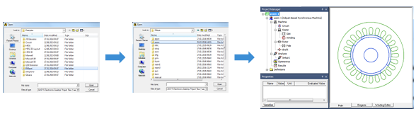
• Open the Electronics Desktop 2016
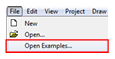
• Open the RMxprtexample ass m1.aedt under File → Open Examples → RMxprt → ass m → ass m1.aedt
• Save the File in a different folder, in order not to modify the default example
RMxprt Model Settings
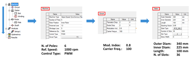
• The model has s mall dimensions and 0.5 kW rated power
– In order to increase machine power, modify the settings as shown in the following pictures, scrolling the machine items/menus from up to down
RMxprt Model Settings
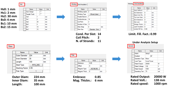
RMxprt Model Settings
– The final machine and the winding setup should look like the ones described in the following pictures
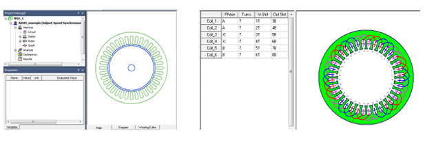
An alysis and Results
– In Project manager window RMB on Setup1 → An alyze to run the simulation
– In Project manager window RMB on Setup1 → Curve to ana lyze results
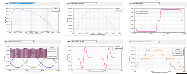
An alysis and Results
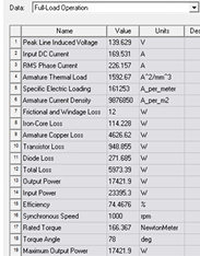
• In Project manager window RMB on Setup1 Performance to an alyze results
• AtFull Load Operation the most important data are:
– Peak Line Induced Voltage:139.6 V
– RMS Phase Current: 226.2 A
– Iron-Core Loss:114.2 W
– Armature Copper Loss:4627 W
– Total Loss:5973.4 W
– Output Power: 17421.9 W
– Input Power: 23395.3 W
– Efficiency:74.47 %
– Torque Angle: 78 deg
– Maximum Output Power: 17421.9 W
Note that efficiency considers also the losses in driving converter RMxprt suggests that 17.4 kW is the maximum power possible to be obtained with that machine
Maxwell Design Creation
• In Project manager window RMB on Setup1 Create Maxwell Design…
• Create both the 2D and the 3D Model
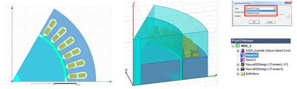
Note that every time a model is created, also the corresponding external circuit is automatically created
Maxwell 2D Design Inspection
• Independently from 2D or 3D, the settings are mostly identical
– Expand the tree for the 2D design and scroll it from up to down to inspect the settings
– Double click on MotionSetup1 and verify the speed is constant at 1000 rpm, starting position is -10 deg and motion type is set to Rotation
– Inspect Boundaries: VectorPotential1 should be set on the external stator side, while Master and Slave are set on the two cut sides.
– Slave must be Bs = -Bm
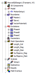

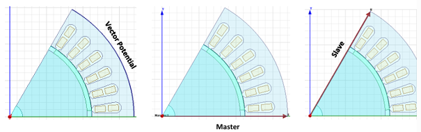
Maxwell 2D Design Inspection
– Double click on PhaseA, PhaseB and PhaseC Windings and verify the sources are set to External and conductors to Stranded
– The winding selection highlights the belonging conductors
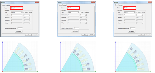
Maxwell 2D Design Inspection
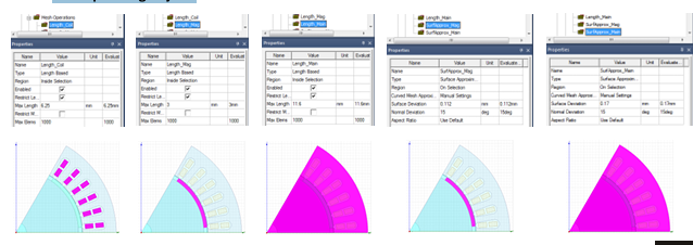
– Click on each Mesh operation an verify the settings are as shown in the following pictures
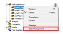
– RMB on each mesh operation Select Assignment highlights the corresponding objects
Maxwell 2D Design Inspection
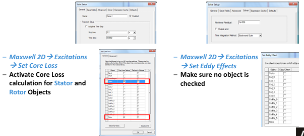
– Double Click on Setup1 an verify the settings are as shown in the following pictures. In Solver Tab
modify the Non linear Residual to 1e-6
更多内容见附件
免责声明:
本页面/内容部分素材来源于互联网公 开 信 息,旨在传递更多信息,不代表本平台立场。
版权归原作者或机构所有,如涉及侵权,请通过平台联系我们,我们将在核实后第一时间处理。
本平台对转载内容的真实性、准确性不作任何保证,用户需自行判断并承担使用风险。