程序员专用 DSP 算法：数学原理与源码实现

4月前浏览502

程序员专用 DSP 算法：数学原理与源码实现（(Dsp) Algorithms For Programmers）

摘要：《(Dsp) Algorithms For Programmers》是一本面向程序员的 DSP 算法与数学原理实战手册，聚焦数字信号处理核心算法的数学原理与代码实现。全书系统讲解离散傅里叶变换、基 2 / 基 4 / 分裂基 FFT、卷积、Z 变换、哈特利变换、数论变换、沃尔什变换、哈尔变换等核心算法，给出递归与非递归实现、三角函数计算优化、内存访问改进及代码自动生成方法。同时涵盖位操作、排列、排序、组合算法、高精度运算等底层技术，提供可直接复用的伪代码与 C++ 源码，兼顾理论推导与工程效率，适合 DSP 开发、算法实现与高性能计算参考。

Algorithms for programmers ideas and source code

This document is work in progress: read the ”important remarks” near the beginning

J¨org Arndt

arndt@jjj.de

This document1 was LATEX’d at September 26, 2002

Some important remarks

about this document.

This draft is intended to turn into a book about selected algorithms. The audience in mind are pro- grammers who are interested in the treated algorithms and actually want to have/create working and reasonably optimized code.

The printable full version will always stay online for free download. It is planned to also make parts of the TEXsources (plus the scripts used for automation) available. Right now a few ﬁles of the TEX sources and all extracted pseudo-code snippets1 are online. The C++-sources are online as part of FXT or hfloat (arithmetical algorithms).

The quality and speed of development does depend on the feedback that I receive from you. Your criticis m concerning language, style, correctness, omissions, technicalities and even the goals set here is very welcome. Thanks to those2 who helped to improve this document so far! Thanks also to the people who share their ideas (or source code) on the net. I try to give due references to original sources/authors wherever I can. However, I am in no way an expert for history of algorithms and I pretty sure will never be one. So if you feel that a reference is missing somewhere, let me know.

New chapters/sections appear as soon as they contain anything useful, sometimes just listings or remarks outlining what is to appear there.

A ”TBD: something to be done” is a reminder to myself to ﬁll in something that is missing or would be nice to have.

The style varies from chapter to chapter which I do not consider bad per se: while some topics (e.g. FFTs) need a clear and explicit introduction others (e.g. the bitwizardry chapter) seem to be best presented by basically showing the code with just a few comments. Still other parts (e.g. sorting) are presented elsewhere extremely well so I will introduce the basic ideas only very shortly and supply some (hopefully) useful code.

Sprache will partly go away: using/including the actual code from FXT will be beneﬁcial to both this document and FXT itself. The goal is to automatically include the functions referenced. Clearly, this will drastically reduce the chance of errors in the shown code (and at the same time drastically reduce the workload for me). Initially I planned to write an interpreter for Sprache, it just never happened. At the same time FXT will be better documented which it really needs. As a consequence Sprache will only be used when there is a clear advantage to do so, mainly when the corresponding C++ does not appear to be self explanatory. Larger pieces of code will be presented in C++. A tiny starter about C++ (some good reasons in favor of C++ and some of the very basics of classes/overloading/templates) will be included. C programmers do not need to be shocked by the ζ++’: only an rather minimal set of the C++ features is used.

The theorem-like environment for the codes shall completely go away. It leads to duplication of state- ments, especially with non-pseudo code (running text, description in the environment and comments at the begin of the actual code).

Enjoy reading !

List of important Symbols

沦x real part of x

$x imaginary part of x

x∗ complex conjugate of x

a a sequence, e.g. {a0 , a1 , ..., an−1}, the index always starts with zero.

a transformed (e.g. Fourier transformed) sequence

m emphasize that the sequences to the left and right are all of length m =

F [a] (= c) (discrete) Fourier transform (FT) of a, ck = Σx(n) 0(1) ax zx k where z = e±2π i/n

F−1 [a] inverse (discrete) Fourier transform (IFT) of a, F−1 [a]k = Σx(n) 0(1) ax z −x k

Ska a sequence c with elements cx := ax e± k 2π ix/n

H [a] discrete Hartley transform (HT) of a

a sequence reversed around element with index n/2

aS the symmetric part of a sequence: aS := a + a

aA the antisymmetric part of a sequence: aA := a − a

Z [a] discrete z-transform (ZT) of a

Wv [a] discrete weighted transform of a, weight (sequence) v

W 1 [a] inverse discrete weighted transform of a, weight v

a ④ b cyclic (or circular) convolution of sequence a with sequence b

a ④ac b acyclic (or linear) convolution of sequence a with sequence b

a ④ − b negacyclic (or skew circular) convolution of sequence a with sequence b

a ④{v} b weighted convolution of sequence a with sequence b, weight v

a ④⊕ b dyadic convolution of sequence a with sequence b

n\N n divides N

n ⊥ m g cd(n, m) = 1

a(j%m) sequence consisting of the elements of a with indices k: k ≡ j mod m e.g.

a(even) , a(odd)a(0%2) , a(1%2)

a(j/m) sequence consisting of the elements of a with indices k: j · n/m ≤ k < (j + 1) · n/m e.g.

a(left) , a(right)a(0/2) , a(1/2)

Chapter 1 The Fourier transform

1.1 The discrete Fourier transform

The discrete Fourier transform (DFT or simply FT) of a complex sequence a of length n is deﬁned as

z is an n-th root of unity: zn = 1.

Backtransform (or inverse discrete Fourier transform IDFT or simply IFT) is then

To see this, consider element y of the IFT of the FT of a:

As Σk (z①__y )k = n for x = y and zero else (because z is an n-th root of unity). Therefore the whole

expression is equal to

where

Here we will call the FT with the plus in the exponent the forward transform. The choice is actually arbitrary1 .

CHAPTER 1. THE FOURIER TRANSFORM

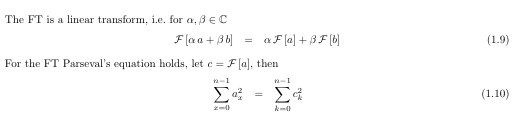
The normalization factor in front of the FT sums is sometimes replaced by a single in front of the inverse FT sum which is often convenient in computation. Then, of course, Parseval’s equation has to be modiﬁed accordingly.

A straight forward implementation of the discrete Fourier transform, i.e. the computation of n sums each of length n requires ~ n2 operations:

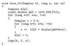
[FXT: slow ft in slow/slowft.cc] is must be +1 (forward transform) or __1 (backward transform), SinCos(x) returns a Complex(cos(x), sin(x)).

A fast Fourier transform (FFT) algorithm is an algorithm that improves the operation count to propor- tional n Σ k __ 1), where n = p1p2 · · · pm is a factorization of n. In case of a power n = pm the value computes to n (p __ 1) logp (n). In the special case p = 2 even n/2 log2 (n) (complex) multiplications suﬃce. There are several diﬀerent FFT algorithms with many variants.

1.2 Symmetries of the Fourier transform

A bit of notation turns out to be useful:

Let a be the sequence a (length n) reversed around element with index n/2:

Let aS , aA be the symmetric, antisymmetric part of the sequence a, respectively

(The elements with indices 0 and n/2 of aA are zero). Now let a ∈ R (meaning that each element of a is ∈ R), then

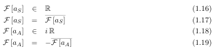
The FT of a real symmetric sequence is real and symmetric and the FT of a real antisymmetric sequence is purely imaginary and antisymmetric. Thereby the FT of a general real sequence is the complex conjugate of its reversed:

Similarly, for a purely imaginary sequence b ∈ iR:

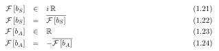
The FT of a complex symmetric/antisymmetric sequence is symmetric/antisymmetric, respectively.

1.3 Radix 2 FFT algorithms

1.3.1 A little bit of notation

Always assume a is a length-n sequence (n a power of two) in what follows:

Let a(even) , a(odd) denote the (length-n/2) subsequences of those elements of a that have even or odd indices, respectively.

Let a(left) denote the subsequence of those elements of a that have indices 0 . . . n/2 __ 1.

Similarly, a(right) for indices n/2 n __ 1.

Let S ka denote the sequence with elements ax e§ k 2π ix/n where n is the length of the sequence a and the sign is that of the transform. The symbol S shall suggest a shift operator. In the next two sections only S 1/2 will appear. S0 is the identity operator.

1.3.2 Decimation in time (DIT) FFT

The following observation is the key to the decimation in time (DIT) FFT2 algorithm: For n even the k-th element of the Fourier transform is

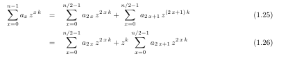
where z = e§i 2π/n and k ∈ {0, 1, , n __ 1}.

The last identity tells us how to compute the k-th element of the length-n Fourier transform from the length-n/2 Fourier transforms of the even and odd indexed subsequences.

To actually rewrite the length-n FT in terms of length-n/2 FTs one has to distinguish the cases 0 ≤ k < n/2 and n/2 ≤ k < n, therefore we rewrite k ∈ {0, 1, 2, . . . , n __ 1} as k = j + δ where j ∈ {0, 1, . . . , n/2 __ 1}, δ ∈ {0, 1}.

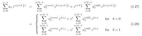
Notingthatz2 is just therootofunitythatappears ina length-n/2FTonecanrewritethe last two equationsasthe

Idea1.1(FFTradix2DITstep)Radix2decimationintimestepfortheFFT:

(Here it is silently assumed that ’+’ or ’__’ between two sequences denotes elementwise addition or subtraction.)

The length-n transform has been replaced by two transforms of length n/2. If n is a power of 2 this scheme can be applied recursively until length-one transforms (identity operation) are reached. Thereby the operation count is improved to proportional n · log2 (n): There are log2 (n) splitting steps, the work in each step is proportional to n.

Code 1.1 (recursive radix 2 DIT FFT) Pseudo code for a recursive procedure of the (radix 2) DIT FFT algorithm, is must be +1 (forward transform) or -1 (backward transform):

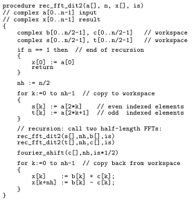
The data length n must be a power of 2. The result is in x []. Note that normalization (i.e. multiplication of each element of x [] by 1/√n) is not included here.

[FXT: recursive dit2 fft in slow/recfft2.cc] The procedure uses the subroutine

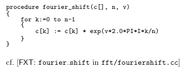
Code 1.2 (Fourier shift) For each element in c[0..n-1] replace c[k] by c[k] times ev 2 π ik/n . Used with U = § 1/2 for the Fourier transform.

The recursive FFT-procedure involves n log2(n) function calls, which can be avoided by rewriting it in

a non-recursive way. One can even do all operations in place, no temporary workspace is needed at

all. The price is the necessity of an additional data reordering: The procedure revbin_permute(a[],n)

rearranges the array a[] in a way that each element ax is swapped with a˜x, where ˜x is obtained from x

by reversing its binary digits. This is discussed in section 8.1.

Code 1.3 (radix 2 DIT FFT, localized) Pseudo code for a non-recursive procedure of the (radix 2)

DIT algorithm, is must be-1 or +1:

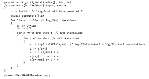
[FXT: dit2-fft-localized in fft/fftdit2.cc]

This version of a non-recursive FFT procedure already avoids the calling overhead and it works in place. It works as given, but is a bit wasteful. The (expensive!) computation e := exp(is*2*PI*I*j/m) is done n/2 · log2 (n) times. To reduce the number of trigonometric computations, one can simply swap the two inner loops, leading to the ﬁrst ζreal world’ FFT procedure presented here:

Code 1.4 (radix 2 DIT FFT) Pseudo code for a non-recursive procedure of the (radix 2) DIT algo- rithm, is must be -1 or +1:

procedure fft_dit2(a [] , ldn, is)

// complex a[0 . .2**ldn-1] input, result

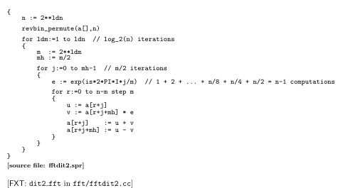
Swapping the two inner loops reduces the number of trigonometric (exp()) computations to n but leads to a feature that many FFT implementations share: Memory access is highly nonlocal. For each recursion stage (value of ldm) the array is traversed mh times with n/m accesses in strides of mh. As mh is a power of 2 this can (on computers that use memory cache) have a very negative performance impact for large values of n. On a computer where the CPU clock (366MHz, AMD K6/2) is 5.5 times faster than the memory clock (66MHz, EDO-RAM) I found that indeed for s mall n the localized FFT is slower by a factor of about 0.66, but for large n the same ratio is in favour of the ζnaive’ procedure!

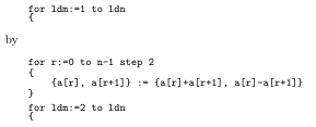
It is a good idea to extract the ldm==1 stage of the outermost loop, this avoids complex multiplications with the trivial factors 1 + 0 i: Replace

更多内容见附件

免责声明：

本页面/内容部分素材来源于互联网公开信息，旨在传递更多信息，不代表本平台立场。

版权归原作者或机构所有，如涉及侵权，请通过平台联系我们，我们将在核实后第一时间处理。

本平台对转载内容的真实性、准确性不作任何保证，用户需自行判断并承担使用风险

电器的定义-电器学的理论范畴

概论概述本课程的主要理论范畴电器技术的国内外现状电器的定义和分类典型电器的结构原理§0-1概述本章教学目的与要求：了解我国电器工业的现状及其发展前景；掌握电器的定义与分类、电器学的理论范畴，对典型电器的原理结构有一定的认识。本章教学重点与难点：电器的定义；电器学的理论范畴本章教学基本内容1、什么是电器？如何分类？2、典型电器结构原理3、电器学的主要理论范畴4、我国电器工业现状及电器发展历史与展望§0-2本课程的主要理论范畴电磁机构理论；电接触理论；电弧理论；发热和电动力理论一、电磁机构理论磁路与电磁铁特性。特点：电器电磁机构是有可动铁心和可变气隙的电磁装置，应用分析软件能正确计算电磁场的分布，由吸力与反力特性曲线关系将能确定电磁机构的形状和尺寸。二、电接触理论目的:触头设计电接触理论包括：（1）电接触的物理化学过程中的热、电、磁以及金属变形等的效应；（2）接触电阻的物理化学本质及其计算；（3）接触或开断过程中，触头的腐蚀、磨损和金属迁移；（4）触头在闭合过程中振动磨损和熔焊。还包括电接触的结构形式、触头材料、加工工艺等。三、电弧理论（1）生弧的物理基础：电离和激励的概念，气体放电和击穿，火花放电、辉光放电和弧光放电的界定和过程等（2）弧柱理论：包含离子平衡的物理化学状态；电弧的直径与温度分布；电弧的弧根和斑点；电弧等离子流；电弧电位梯度（3）电弧的静伏安特性和动伏安特性；（4）电弧过零时的介质恢复和电压恢复过程。、四、发热和电动力理论1.发热计算：发热损耗计算；交流电器因集肤效应和邻近效应产生的涡流和磁滞附加损耗导致的发热计算；电器在不同工作制下的发热计算；导电部件在大电流下的发热计算，以及热稳定性校验。2.电动力计算：不同几何位置安置的导体间电动力的分析和计算。§0-3电器技术的国内外现状——我国的电器工业发展历程：仿苏→自己研发→引进、消化先进技术产业现状：三分天下（私营企业、国营企业、外企）课堂花絮:播放正泰、北开（厂长黄国诚为我校校友）、桂林电科所等若干企业的资料片。讨论：为何我国大部分电器产品质量不如国外产品？§0-4电器的定义和分类一、电器的定义凡根据外界指定信号和要求，自动或手动接通或断开电路，断续或连续地改变电路参数，以实现对电路或非电对象切换、控制、保护、检测、变换和调节用的电气设备，称为电器。二、电器的分类1、工作职能:手动、自动、起动调速、稳压与调压、测量放大与变换、牵引与传动;2、结构工艺和生产部门:高压、低压、自动电磁元件、成套电器与自动化装置;3、元件与使用系统的关系：电力网系统用、电拖系统用、自动化通讯用；4、使用场合和工作条件：一般工业、特殊工况、农用、热带电器与高原电器、船用航空牵引用;5、执行机能和转换深度：有触点、无触点和混合式电器等。§0-5典型电器的结构原理一、继电器类型：电磁式与非电磁式（气囊式、受热等）;名称:电流继电器、电压继电器、热继电器、时间继电器、光继电器、压力继电器、速度继电器等。结构：感测元件、操动机构、辅助触头。特性（1）继电特性:反映继电器的输出—输入关系的特性。可用右图表示。Xl是继电器的动作值XR是继电器的返回值（2）吸合值与释放值；（3）返回系数；（4）动作灵敏度（规定负载下的最小动作功率）；（5）动作时间。二、接触器类型：直流接触器、交流接触器。（1）直流接触器主触头为单断点转动式，上装灭弧室；辅助触头随衔铁一同动作。线圈通电后，衔铁克服反力闭合；线圈断电，衔铁释放。（2）交流接触器作用：通断交流主电路，以三相为主，也有四相。结构：线圈电源是交流或直流；形式上有转动式和直动式，右图为转动式。还有辅助触头和采用磁吹、窄缝和删片等灭弧原理的灭弧室。下图为直动式交流接触器。其主触头是双断口，材料为银基合金。（3）真空接触器动静触头真空泡真空介质电磁操动机构三、各类接触器实物图免责声明：本页面/内容部分素材来源于互联网公开信息，旨在传递更多信息，不代表本平台立场。版权归原作者或机构所有，如涉及侵权，请通过平台联系我们，我们将在核实后第一时间处理。本平台对转载内容的真实性、准确性不作任何保证，用户需自行判断并承担使用风险。