ANSYS Aqwa 理论手册15.0(Aqwa Theory Manual)

摘要:
本文为 ANSYS Aqwa 15.0 官方理论手册,系统阐述海洋工程结构水动力分析的完整理论体系。手册先明确坐标系、波浪 / 风 / 流环境建模方法,涵盖规则波、二阶 Stokes 波、多种波浪谱及风场、流速剖面定义;再讲解浮体静水力、稳性与刚度矩阵计算,基于源汇法开展辐射 / 绕射分析,处理附加质量、阻尼与 RAO 求解。同时介绍二阶波浪力、QTF、平均漂移力及 Morison 方程、系泊系统、铰接约束、护舷、锚缆与拖缆建模,支持频域 / 时域仿真,适用于船舶、海洋平台等结构运动与载荷分析,为海洋工程水动力仿真提供权威理论依据。
Copyright and Trademark Information
© 2013 SAS IP, Inc. All rights reserved. Unauthorized use, distribution or duplication is prohibited.
ANSYS, ANSYS Workbench, Ansoft, AUTODYN, EKM, Engineering Knowledge Manager, CFX, FLUENT, HFSS and any and all ANSYS, Inc. brand, product, service and feature names, logos and slogans are registered trademarks or
trademarks of ANSYS, Inc. or its subsidiaries in the United States or other countries. ICEM CFD is a trademark used by ANSYS, Inc. under license. CFX is a trademark of Sony Corporation in Japan. All other brand, product, service
and feature names or trademarks are the property of their respective owners.
Disclaimer Notice
THIS ANSYS SOFTWARE PRODUCT AND PROGRAM DOCUMENTATION INCLUDE TRADE SECRETS AND ARE CONFID-
ENTIAL AND PROPRIETARY PRODUCTS OF ANSYS, INC., ITS SUBSIDIARIES, OR LICENSORS. The software products
and documentation are furnished by ANSYS, Inc., its subsidiaries, or affiliates under a software license agreement
that contains provisions concerning non-disclosure, copying, length and nature of use, compliance with exporting
laws, warranties, disclaimers, limitations of liability, and remedies, and other provisions. The software products
and documentation may be used, disclosed, transferred, or copied only in accordance with the terms and conditions of that software license agreement.
ANSYS, Inc. is certified to ISO 9001:2008.
U.S. Government Rights
For U.S. Government users, except as specifically granted by the ANSYS, Inc. software license agreement, the use, duplication, or disclosure by the United States Government is subject to restrictions stated in the ANSYS, Inc.
software license agreement and FAR 12.212 (for non-DOD licenses).
Third-Party Software
See the legal information in the product help files for the complete Legal Notice for ANSYS proprietary software and third-party software. If you are unable to access the Legal Notice, please contact ANSYS, Inc.
Published in the U.S.A.
Chapter 1: Introduction to Aqwa Solver Theory
ANSYS® Aqwa™ provides a toolset for investigating the effects of environmental loads on floating and fixed offshore and marine structures. This includes, but is not limited to, floating production and offload- ing systems, spars, semi-submersibles, renewable energy systems, and ships.
This document provides a description of the theoretical basis of this product.
1.1. Aqwa General Capabilities
Aqwa can simulate linearized hydrodynamic fluid wave loading on floating or fixed rigid bodies. This
is accomplished by employing three-dimensional radiation/diffraction theory and/or Morison’s equation in regular waves in the frequency domain. Unidirectional or multiple directional second order drift forces are evaluated by the far-field, or near field solution, or full quadratic transfer function (QTF) matrix. Free- floating hydrostatic and hydrodynamic a nalyses in the frequency domain can also be performed.
Aqwa can estimate the equilibrium characteristics and static and dynamic stability of coupled (by
moorings and/or connectors) bodies under steady state environmental loads (e.g. wind, wave drift and current).
Aqwa can perform frequency domain statistical an alysis of the coupled or uncoupled responses of
floating bodies while operating in irregular waves. The linearized drag due to Morison elements (tube, disc), wind and dynamic cables can also be simulated in Aqwa.
The real-time motion of a floating body or bodies while operating in regular or irregular waves can be simulated, in which nonlinear Froude-Krylov and hydrostatic forces are estimated under instantaneous incident wave surface. Additionally, the real-time motion of a floating body or bodies while operating in multi-directional or unidirectional irregular waves can be simulated under first- and second-order
wave excitations. Wind and current loading can also be applied to the bodies, as well as external forces at each time step imported or defined by a user-written dynamic-link library. If more than one body is being studied, coupling effects between bodies can be simulated. The convolution approach is used
to account for the memory effect of the radiation force.
Wave loads on fixed or floating structures calculated during radiation/diffraction simulation in Aqwa can be mapped to a finite element structural an alysis package. Specific details of this procedure are not included in this document.
1.2. Axes Conventions
Various coordinate systems are employed in Aqwa for representing motions, loads, and other vector
values. The general transformation matrix between different coordinate systems and the Euler trans-
formation matrix as a special case are described in this section. The fixed reference axes (FRA), local
structure axes (LSA) and local articulation axes are also described in this section. Other Aqwa-used axis frames, such as local axis systems for tether elements and tube elements, will be described in more
detail in subsequent chapters.
1.2.1. Fixed Reference Axes
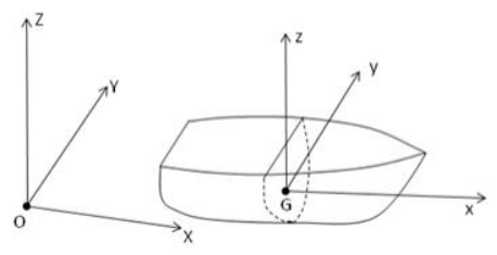
In hydrodynamic problems that include a fluid free-surface boundary, it is common practice to define a system of axes with the origin in the mean free surface of the fluid, as shown in Figure 1.1: Definition of Axis Systems (p. 2). In Aqwa this is referred to as the fixed reference axes (FRA), global axes, or
OXYZ, which is a fixed right handed axis system with the origin in the mean free surface and Z-axis pointing vertically upwards.
Figure 1.1: Definition of Axis Systems
1.2.2. Local Structure Axes
For the description of rigid body motions, it is more convenient to use the center of gravity of the body as a dynamic reference point. The local structure axes (LSA), body fixed axes, or Gxyz, is defined for
each individual structure. As shown in Figure 1.1: Definition of Axis Systems(p. 2), the origin of the local structure axes is at the body's center of gravity. The local structure axes through the center of gravity will initially be parallel to the fixed reference axes.
1.2.3. Local Articulation Axes
Aqwa allows structures to be connected by articulated joints. These joints do not permit relative trans- lation of the two structures but allow relative rotational movement in a number of ways that can be
defined by the user. The local articulation axes (LAA) or Axyz is shown in Figure 1.2: Local Articulation Axes (p. 3).
Figure 1.2: Local Articulation Axes
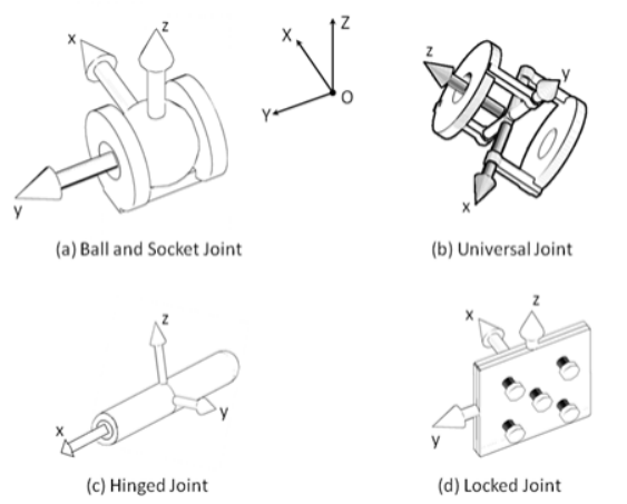
The local articulation axes are a local right handed coordinate system based on the following constraint types:
Ball and Socket Joint:
The origin is located at the connecting point, with the local x-, y-, and z-axes parallel to the X-, Y-, and Z-axes of the FRA at the initial position.
Universal Joint:
The origin is located at the connecting point, with the local x- and y-axes parallel to the two freely rota- tional freedoms. The local z-axis is at right angles to the local x- and y-axes.
Hinged Joint:
The origin is located at the connecting point, with the local x-axis parallel to the hinge axis. The local y- axis is at right angle to the local x-axis and in the OXY plane of the FRA at the initial position. In cases where the hinge axis is parallel to the Z-axis of the FRA in the initial position, the local y-axis will be
parallel to the Y-axis of FRA.
Locked Joint:
The origin is located at the connecting point, with the local x-, y- and z-axes parallel to the X-, Y- and Z-axes of the FRA at the initial position.
1.2.4. Axis Transformation and Euler Rotations
Position, velocity, acceleration and force are represented in Aqwa by vectors with both magnitude and direction. These vectors can be described in the different coordinate systems by means of an axis transformation.
Figure 1.3: Axis Transformation
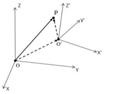
Figure 1.3: Axis Transformation(p. 4) shows two coordinate systems, the origin of the O'X'Y'Z' frame
is at [X0, Y0, Z0]T in the OXYZ frame, where the superscript T denotes a matrix transpose. The directional cosines of the O'X'Y'Z' axes relative to the OXYZ axes are written as

If the coordinate of a point is represented as [X, Y, Z]T in OXYZ and [x, y, z]T in O'X'Y'Z', then we have

where is the transformation matrix.
To transfer [X, Y, Z]T in OXYZ into a coordinate in the O'X'Y'Z' frame, we have

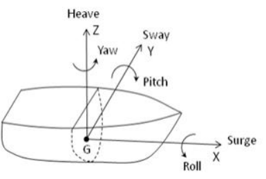
Employing the conventional seakeeping notation of a floating rigid body (see [25]), motions of that
body are defined as the translational movements of the center of gravity and rotations about a set of
orthogonal axes through the center of gravity, GXYZ, as illustrated in Figure 1.4: Floating Rigid Motions
(p. 5). This intermediate coordinate system moves with the mean forward speed of the vessel but its
X-, Y-, and Z-axes remain constantly parallel to the corresponding X-, Y-, and Z-axes of the fixed reference axes.
Figure 1.4: Floating Rigid Motions
Translations
u1 = surge (along X)
u2 = sway (along Y)
u3 = heave (along Z)
Rotations
θ1 = roll (about X)
θ2 = pitch (about Y)
θ3 = yaw (about Z)
The naming of the various motions assumes that the body is described such that the forward and aft direction is parallel to the X-axis. If the body lies parallel to the Y-axis, then the rolling of the body will be termed 'pitch' and the pitching termed 'roll'.
For large amplitude rotational motion an alysis, determination of Euler angles is a necessary step in kinematics and model graphic presentation. Aqwa defines the orientation of a structure using Euler angles. These are the rotation angles about the three axes of GXYZ:
A rotation of θ1 about the X-axis:

A rotation of θ2 about the Y-axis:

A rotation of θ3 about the Z-axis:

The Euler rotation matrix is defined as a sequence of three rotations, in the order of the rotation first about the X-axis of GXYZ, then the Y-axis, and finally the Z-axis of GXYZ. It can be represented as the matrix product:

With this Euler rotation matrix, similar to Equation 1.2 (p. 4), the position of a point in the fixed reference axes can be expressed as

where (Xg, Yg, Zg)T is the coordinate of the center of gravity in the fixed reference axes and (x, y, z)T is the coordinate of this point in the local structure axes (LSA).
As a special case when all the rotational angles are s mall, for instance θj = O ε j = 1 , 3) , the Euler rotation matrix can be simplified to:

where


1.3. Direction and Phase Angle Conventions
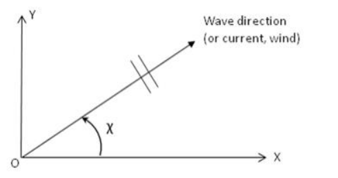
The wave, current and wind directions are defined in the OXY plane of the fixed reference axes (FRA). The direction is defined as the angle between the wave, current, or wind propagating direction and the positive X-axis measured anti-clockwise, as shown in Figure 1.5: Direction Definition(p. 7). For ex- ample, the heading angle is 0 when the wave propagation is along the positive X-axis of the global axes (following wave) and 90 when along the positive Y-axis of the global axes (beam wave).
Figure 1.5: Direction Definition
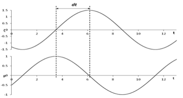
The phase angle of a parameter, such as the surge response amplitude operator (RAO) or wave exciting force, is defined according to the difference from the time when the regular wave crest is at the center of gravity of a structure to the time when this parameter reaches its peak value. In other words, the
time histories of an incident wave elevation and a corresponding force or response parameter are rep- resented in the fixed reference axes as

where aw is the regular wave amplitude, ⑴ is the wave frequency (in rad/s), α is the wave phase angle (in radians) relative to the origin of the fixed reference axes, ap is the amplitude of the parameter, and is the phase angle of the parameter (in rad/s). The phase angle in degrees is given by:

As shown in Figure 1.6: Phase Definition(p. 7), a positive phase angle indicates that the parameter lags behind the wave.
Figure 1.6: Phase Definition
Chapter 2: Ocean Environmental Conditions
Information on ocean environmental conditions, such as winds, waves and current, is critical for the
design of all types of marine structures, and is especially important for floating offshore structures for which hydrodynamic behavior in open sea is more complicated than fixed structures. Waves apply ex- citing forces at wave frequency and nonlinear wave forces (for example, low frequency drift force and sum frequency second order forces), or alternatively nonlinear wave forces due to variation of the in- stantaneous wetted hull surface. Winds and current cause forces on the exposed members of the
structure above and below the water surface respectively, and the forces are generally evaluated in Aqwa by a nonlinear drag force term.
This chapter describes the numerical models of waves, wind, and current available in Aqwa.
2.1. Ocean Waves
Ocean waves are composed of waves with different frequencies and directions. The waves from different directions interact and cause wave conditions to be very difficult to model mathematically. Various
simplified theories and wave spectral models of ocean waves are introduced in the literature, such as s mall amplitude linear Airy wave, higher order Stokes wave, and irregular waves represented by wave spectra.
Aqwa can simulate first order (Airy wave) and second order (2nd order Stokes wave) regular waves in deep and finite depth water. Additionally, unidirectional or multi-directional irregular waves can be
modeled by using the linear superposition approach.
2.1.1. Regular Wave
This section provides a brief description of the linear regular wave (Airy wave) and the second order Stokes wave in either deep water or finite depth water.
2.1.1.1. Linear Regular Wave
Linear wave (Airy wave) is considered as the simplest ocean wave, and is based on the assumption of homogeneous, incompressible, inviscid fluid and irrotational flow. In addition, the wave amplitude is assumed to be s mall compared to the wave length and water depth; hence the linear free surface
condition is used.
In the fixed reference axes (FRA), the water surface elevation at position X and Y can be expressed in complex value form as
ζ =a wei [ _⑴ t +k(xcosx +y si"x)+α ] (2.1)
where aw is the wave amplitude, ⑴ is the wave frequency (in rad/s), k is the wave number, x is the wave propagating direction, and α is the wave phase.
Assuming ideal, irrotational fluid, the flow can be represented by a velocity potential satisfying the
Laplace equation in the whole fluid domain, the linear free surface condition, and horizontal impermeable bottom condition.



where d is water depth and g is gravitational acceleration.
Employing the linear free surface condition, the relationship between the wave frequency and the wave
number (the linear dispersion relationship) is represented by

The wave length and wave period are

Using the Bernoulli equation and only taking account the linear term, the fluid pressure is

where p is the water density.
The wave celerity is

 (2.6)
(2.6)
Taking the partial derivative of the velocity potential, the fluid particle velocity is

When the wave particle velocity at the crest equals the wave celerity, the wave becomes unstable and begins to break (see [24]). The limiting condition for wave breaking in any water depth is given by:

In infinite depth water (d → ∞), the wave elevation keeps the same form as Equation 2.1 (p. 9), but velocity potential is further simplified as
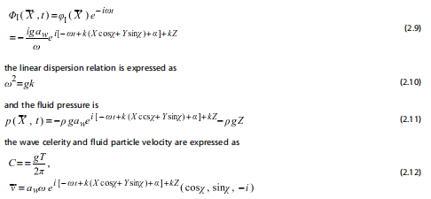
From Equation 2.8 (p. 10), for deep water wave, the wave breaks when the wave height (aw) is 1/7th of the wave length.
2.1.1.2. Second Order Stokes Wave
Advanced wave theories may be necessary in some cases when the nonlinearities are important (see
[4] and [8]). Aqwa allows application of the second order Stokes wave theory for moderate or severe
regular wave conditions when the nonlinear Froude-Krylov force over the instantaneous wetted surface is estimated.
Choosing the ratio of the wave amplitude to wave length as the s mallness parameter ε, Taylor expansions for the velocity potential and wave surface elevation in ε can be written as

For water of finite depth, the second order Stokes wave is expressed as


where X =Xcosx + ysinx.
When the set-down in the second-order Stokes waves is included, the potential and wave elevation are
written as

where

The above new terms are negative constants called set-down, which represent the mean level in regular Stokes waves.
The velocity of a fluid particle at coordinates (X, Y, Z) is

The fluid pressure up to the second order is

Comparing with the linear Airy wave, the second order Stokes wave profile shows higher peaked crests and shallower, flatter troughs.
For deep water cases (d → ∞), the second order Stokes wave given in Equation 2.15 (p. 12) becomes


ζ X Y t = ζ ( 1) X Y t + ζ (2) X Y t

Note that in deep water, the second order Stokes wave potential only consists of the first order com- ponents, and there is no set-down term.
2.1.2. Irregular Waves
Most energy at the ocean surface is contributed by wind generated waves, which usually result from
the wind blowing over a vast expanse of fluid surface. A wind sea is the wind induced wave system
which is directly being generated and affected by the local winds, while a swell consists of wind generated waves that are hardly affected by the local wind at that time but have been generated elsewhere or
some time ago. Full-development sea waves are in a state where the largest of the waves in the sea cannot grow any larger and its wave height and wavelength have reached the full potential.
In practice, the linear theory is used to express the multi-directional sea waves (short crested waves) as the summation of a large number of wave components, for instance:

where Nd and Nm are the number of wave directions and number of wave components along each wave direction xm m = Nd , ajm is the wave amplitude, ⑴jm is the wave frequency, kjm is the wave number, and α jm is the random phase angle of a wave component J m J = NM ) .
The wave representation for irregular seas can be achieved by specification of wave spectra. Mathem- atically speaking, the wave spectrum spreads from zero to infinite frequencies. However, examination of the spectrum shows that the wave energy is often concentrated in a relatively narrow band, which determines the actual wave pattern. Employing characteristic, the summation given in Equa-
tion 2.19 (p. 13) could numerically consist of a limited number of wave components, starting from a
non-zero lower bounded frequency and finishing at a finite-value upper bounded frequency. The selection of these starting and finishing frequencies should ensure that this truncated frequency range covers at
least 99% of overall wave energy.
If a wave spectrum, S m ⑴ , is introduced for the m-th sub-directional waves, the wave amplitude ajm
can be expressed as

Uni-directional waves (Nd= 1) are also called long-crested waves, which propagate along one specified direction only.
Aqwa can accept formulated wave spectrum, user-defined wave spectrum or import time history of wave elevation, and any combination thereof to describe an irregular sea.
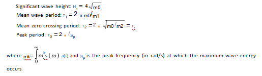
The following wave spectral parameters may be useful:
2.1.2.1. Formulated Wave Spectra
There are several pre-configured wave spectra that only require knowledge of a couple of statistical parameters to fully define the sea state. These are explained below.
2.1.2.1.1. JONSWAP Spectrum
The JONSWAP (Joint North Sea Wave Project) spectrum can take into account the imbalance of energy
flow in the wave system (for instance, when seas are not fully developed). Energy imbalance is nearly
always the case when there is a high wind speed. Parameterization of the classic form of the JONSWAP
spectrum (using fetch and wind speed) was undertaken by Houmb and Overvik [14]. The peak frequency as well as empirical parameters ? and α are used in this formulation. The spectral ordinate at a frequency is given by

where
⑴p is the peak frequency in rad/s, ? is the peak enhancement factor,α is a constant that relates to the wind speed and the peak frequency of wave spectrum, and

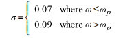
Because α is a constant, the integration of this spectrum can be expressed as

Therefore if ?, ⑴p, and Hs are known, then the variable α can be determined by

You can define the starting and finishing frequencies of the JONSWAP spectrum used in Equa- tion 2.21 (p. 14). By default, Aqwa gives the definitions as:
Starting frequency (in rad/s):

Finishing frequency (in rad/s):
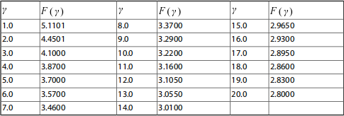
✑f= ✑p .F ✓ (2.25)
where the weighting function values against ✖ ∈ [1 .0 , 20 .0] are listed in Table 2.1: Weighting Function Values (p. 15).
Table 2.1: Weighting Function Values
详细内容请见附件
免责声明:
本页面/内容部分素材来源于互联网公 开 信 息,旨在传递更多信息,不代表本平台立场。
版权归原作者或机构所有,如涉及侵权,请通过平台联系我们,我们将在核实后第一时间处理。
本平台对转载内容的真实性、准确性不作任何保证,用户需自行判断并承担使用风险。