波浪传播与波-结构相互作用CFD模拟的关键影响因素与最佳实践

Prediction of Wave Propagation and Wave‐Structure Interaction
摘要:
本文围绕波浪传播与波 — 结构相互作用的 CFD 模拟,系统分析影响计算精度的关键因素并给出最佳实践。文档指出,一阶时间离散会显著衰减波幅,必须采用二阶格式;网格分辨率与纵横比直接影响波形保真,陡波宜用纵横比 2,中等陡波可用 4。HRIC 格式角度因子、界面耗散、湍流模型及初始边界条件均显著影响结果,低 Re k-ε 模型配合特定初始化可抑制湍黏度异常增长。文末给出波生成、边界处理、阻尼与强制方案的标准化设置,为 STAR-CCM + 波浪仿真提供可靠参数与流程规范。
Introduction
• Problems often encountered with waves
• Factors that affect prediction of wave propagation
• Wave damping
• Forcing solution with waves
• Turbulence and waves
• Some good examples
• Amplitude reduction;
• Disturbances of free surface;
• Reflection at boundaries, etc …
Waves Considered: Wave 1
Wave height: H = 0.14 m
Wavelength: λ = 3.5667 m; Wave steepness: H/ λ ≈ 0.04
Wave period: T = 1.5 s
Water depth: d = 5 m
Δx = 0.03125 m (ca. 114 cells per wavelength)
Δz = 0.0078125 m (ca. 18 cells per wave height) Aspect ratio: Δx/Δz = 4
Time step: 0.005 s (300 time steps per wave period)
Under_relaxation parameters: 0.8 for velocities, 0.4 for pressure, 0.8 for volume fraction Outer iterations per time step: 10 (not optimized for efficiency, rather conservative)
Inviscid, laminar or turbulent flow Second_order time discretization
Second_order space discretization
Gradients: Hybrid Gauss_LSQ, unless otherwise stated
Initial conditions: Stokes 5th_order wave theory
Boundary conditions: Stokes 5th_order wave at inlet, damping at outlet over 2λ
Waves Considered: Wave 2
Wave height: H = 4 m
Wavelength: λ = 47.154 m; Wave steepness: H/ λ ≈ 0.085
Wave period: 5.304 s
Water depth: 77.2 m
Solution domain length: 285 m or 190 m
Δx = 0.5 m (94 cells per wavelength)
Δz = 0.25 m (16 cells per wave height) Aspect ratio: Δx/Δz = 2
Time step: 0.01 s (530 time steps per wave period) Inviscid, laminar or turbulent flow
Second_order time discretization
Second_order space discretization
Gradients: Hybrid Gauss_LSQ, unless otherwise stated
Initial conditions: Stokes 5th_order wave theory
Boundary conditions: Stokes 5th_order wave at inlet, damping at outlet (long domain), or Stokes 5th_order wave at inlet and outlet with forcing over one wavelength
Waves Considered: Wave 3Wave height: H = 0.06 m
Wavelength: λ = 0.8 m; Wave steepness: H/ λ = 0.075
Wave period: T = 0.7 s
Water depth: d = 5 m
Δx = 0.01 m (80 cells per wavelength)
Δz = 0.005 m (12 cells per wave height) Aspect ratio: Δx/Δz = 2
Time step: 0.003 s (233 time steps per wave period)
Under_relaxation parameters: 0.8 for velocities, 0.4 for pressure, 0.8 for volume fraction Outer iterations per time step: 10 (not optimized for efficiency, rather conservative)
Inviscid, laminar or turbulent flow Second_order time discretization
Second_order space discretization Gradients: Hybrid Gauss_LSQ
Initial conditions: Stokes 5th_order wave theory
Boundary conditions: Stokes 5th_order wave at inlet, damping at outlet over 2λ
Factors Affecting Waves• Time discretization
• Grid resolution
• Grid aspect ratio
• Angle factor in HRIC_scheme
• Limiters
• Interface Momentum Dissipation model
• Turbulence model
• Initial and boundary conditions for turbulence
Effects of Time Discretization, I• First_order implicit Euler scheme damps wave amplitude severely and thus cannot be used to simulate wave propagation.
• Second_order quadratic fully_implicit scheme provides a time_ accurate simulation of wave propagation, but imposes a limit on time_step size.
• Free surface should not move more than 40% of cell size in any direction (fitting parabola causes under_ and overshoots).
• This causes often problems if s mall cells are present within free_ surface zone …

Effects of Time Discretization, II
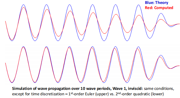
Simulation of wave propagation over 10 wave periods, Wave 1, inviscid: same conditions, except for time discretization – 1st_order Euler (upper) vs. 2nd_order quadratic (lower)
Grid Effects, I• Insufficient number of cells per wavelength and wave height leads to reduced accuracy, as expected.
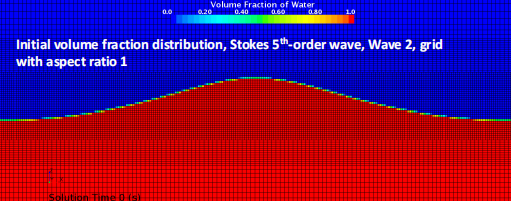
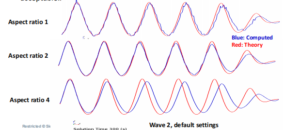
• Cell aspect ratio has a surprisingly high influence on the solution …
• The problem appears to be linked to the fact that the profile of volume fraction is differently “sharp” in different directions …
Grid Effects, II
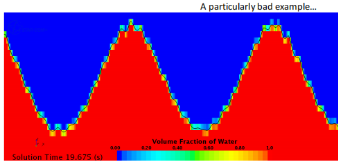
• The HRIC_scheme tries to sharpen the volume fraction transition in x_ direction and thus, for aspect ratio 1, leads to the formation of steps …
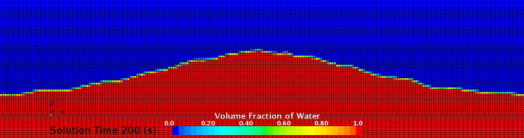
Solution after 38 wave periods, obtained on a grid with aspect ratio 1. There are 236 cells per wavelength, 20 cells per wave height, 530 time steps per wave period (Wave 2 with slightly finer grid – Δz = 0.2 m instead of 0.25 m). The solution domain is over 6 wavelengths long and damping is applied over last 2λ .
Grid Effects, III
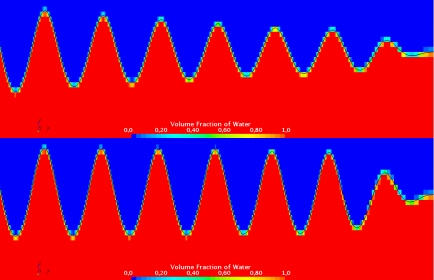
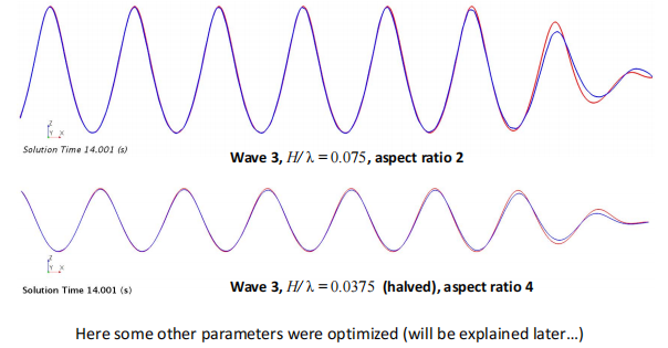
• For steep waves (H/λ > 0.04), aspect ratio of 2 gives best results.
• For waves of s mall to moderate steepness, aspect ratio of 4 is also acceptable …
Grid Effects, IV
Effects of Angle Factor in HRIC_Scheme
• The HRIC_scheme has one parameter called “Angle factor”, whose default value is 0.05; it appears that higher values (0.15 to 0.2) are better for waves.
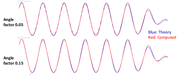
Wave 1, inviscid: Solution after 13.3 wave periods, obtained on a grid with aspect ratio 4
Limiter Effects
• The limiter used in the discretization method also affects the solution...
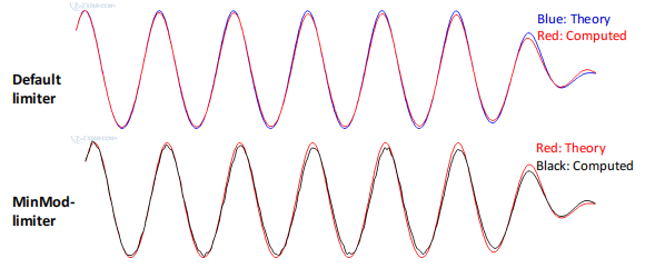
Wave 1, inviscid: Solution after 13.3 wave periods, obtained using different limiters (all other parameters are the same).
Effects of Interface Momentum Dissipation
• The Interface Momentum Dissipation (IMD) model in VoF also affects the solution...
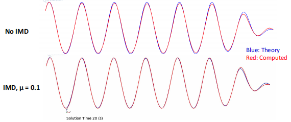
Wave 1, inviscid: Solution after 13.3 wave periods, obtained with and without IMD (all other parameters are the same).
Effects of Turbulence, I
• The choice of both turbulence model and the initial and boundary conditions affects simulations of wave propagation.
• Sylvain Lardeau showed that RANS_models normally lead to growth of turbulent viscosity over time (exponentially!) …
• Only standard low_Re k-ε turbulence model has a built_in term which
will prevent that growth if the initial conditions are such that the ratio of turbulent kinetic energy production over dissipation is < 1.
• However, it appears that this ratio is larger than 1 in the cells that are partially filled with liquid, no matter how turbulence variables are
initialized …
• … which therefore eventually leads to the growth of turbulent viscosity; the initialization decides how long it will take for the effect to become significant …
Effects of Turbulence, II
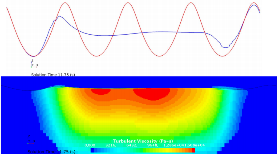
Wave 2, turbulent, low_Re k-ε: Solution after 2.2 wave periods, obtained when starting with default initialization for k and ε (0.001 and 0.1, respectively). Forcing over 1λ applied at both ends, wave propagation from left to right.
Effects of Turbulence, III
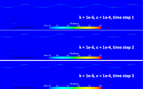
Wave 2, turbulent, low_Re k-ε: Development of Pk/ε over time for one set of initial values
Effects of Turbulence, IV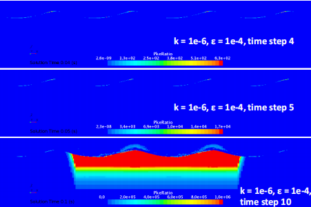
Wave 2, turbulent, low_Re k-ε: Development of Pk/ε over time for one set of initial values
Effects of Turbulence, V
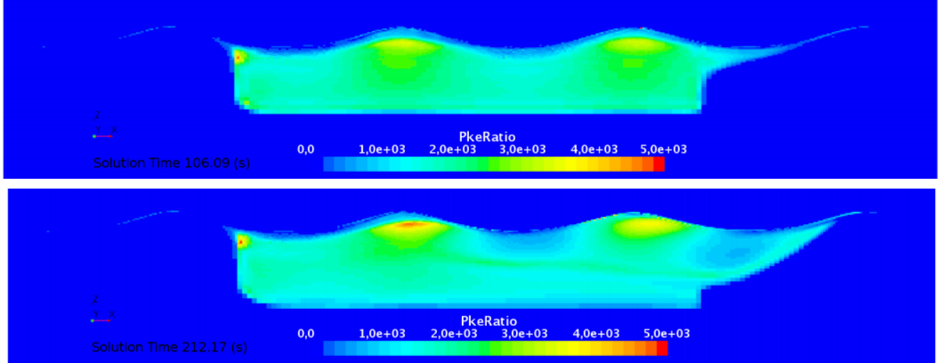
Wave 2, turbulent, low_Re k-ε: Development of Pk/ε over time. For this set of initial values, the ratio of production to dissipation of turbulence does not grow over 5000; in particular, it does not increase substantially after 20 wave periods of simulation. However, turbulent viscosity grows further even for the constant ratio when it is > 1.
Effects of Turbulence, VI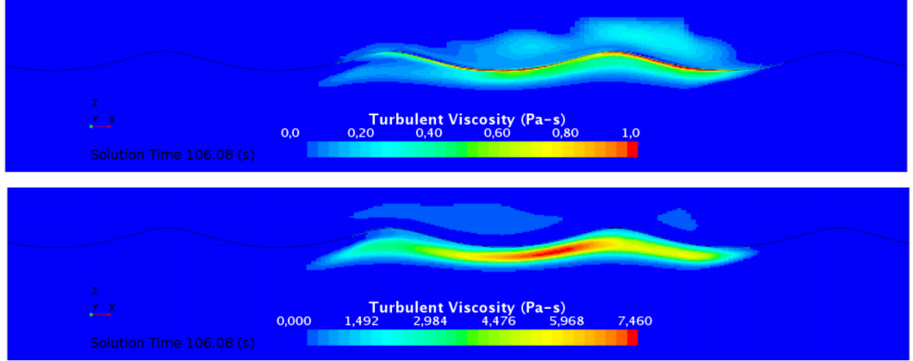
Wave 2, turbulent, low_Re k-ε: Turbulent viscosity after 20 wave periods, obtained when starting with different initializations for k and ε . Best results are obtained for k = 1e_5 and ε = 1e_4. Forcing over 1λ applied at both ends, wave propagation from left to right.
Effects of Turbulence, VII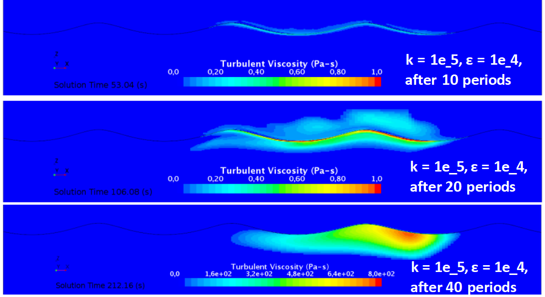
Wave 2, turbulent, low_Re k-ε: Development of turbulent viscosity over time for one set of initial values. Up to 20 wave periods, values are still s mall (up to 1 Pa s), but after another 20 wave periods, turbulent viscosity becomes too high (up to 800 Pa s) …
Effects of Turbulence, VIII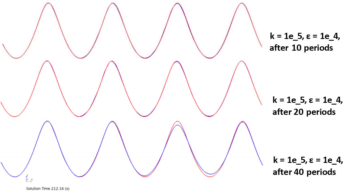
Wave 2, turbulent, low_Re k-ε: Comparison of computed (blue) and theoretical (red) free surface profiles. Once turbulent viscosity becomes high, wave amplitude is reduced …
免责声明:
本页面/内容部分素材来源于互联网公 开 信 息,旨在传递更多信息,不代表本平台立场。
版权归原作者或机构所有,如涉及侵权,请通过平台联系我们,我们将在核实后第一时间处理。
本平台对转载内容的真实性、准确性不作任何保证,用户需自行判断并承担使用风险。