有限元方法:理论基础与核心原理-电子书-723页

有限元方法:理论基础与核心原理(The-Finite-Element-Method--its-Basis-and-Fundamentals)
摘要:
本书是有限元方法理论基础的经典权威著作(第七版),系统阐述有限元法的数学原理、离散流程与工程应用。全书从标准离散系统出发,讲解弱形式、变分原理、加权残差法等核心理论,推导一维 / 多维弹性力学、场问题的有限元列式,介绍拉格朗日与赛尔维普单元、等参映射、高斯积分等关键技术。书中深入分析单元收敛性、分片试验、约束处理、混合元与增强应变元,覆盖自适应网格、误差估计、NURBS 网格生成及瞬态问题求解方法,配套 FEAPpv 程序与大量案例,为有限元理论研究与工程仿真提供完整理论框架和实践指导。
The Finite Element Method: Its Basis and Fundamentals Seventh Edition
O.C. Zienkiewicz, CBE, FRS
Previously UNESCO Professor of Numerical Methods in EngineeringInternational Centre for Numerical Methods in Engineering, Barcelona Previously Director of the Institute for Numerical Methods in Engineering University of Wales Swansea
R.L. Taylor
Professor in the Graduate School Department of Civil and Environmental Engineering University of California at Berkeley
Berkeley, California
J.Z. Zhu
Senior Scientist
ESI US R & D
9891 Broken Land Parkway, Suite 200 Columbia, Maryland
The Finite Element Method: Its Basis and Fundamentals
Professor O.C. Zienkiewicz, CBE, FRS, FREng died on 2 January 2009. Prior to his
death he was Professor Emeritus at the Civil and Computational Engineering Centre, University of Wales, Swansea and previously Director of the Institute for Numerical Methods in Engineering at the University of Wales, Swansea, UK. He also held the UNESCO Chair of Numerical Methods in Engineering at the Technical University of Catalunya, Barcelona, Spain. He was the head of the Civil Engineering Department at the University of Wales, Swansea between 1961 and 1989. During this period he established that department as one of the primary centers of finite element research. In 1968 he became the Founder Editor of the International Journal for Numerical Methods in Engineering which still remains today the major journal in this field. The recipient of 27 honorary degrees and many medals, Professor Zienkiewicz was a member of five academies—an honor he received for his many contributions to the fundamental developments ofthe finite element method. In 1978, he became a Fellow of the Royal Society and the Royal Academy of Engineering. This was followed by his election as a foreign member to the U.S. Academy of Engineering (1981), the Polish Academy of Science (1985), the Chinese Academy of Sciences (1998), and the National Academy of Science, Italy (Academia dei Lincei) (1999). He published the first edition of this book in 1967 and it remained the only book on the subject until 1971.
Professor R.L. Taylor has more than 50 years’ experience in the modeling and simulation of structures and solid continua including eight years in industry. He is Professor of the Graduate School and the Emeritus T.Y. and Margaret Lin Professor of Engineering at the University of California at Berkeley and Corporate Fellow at Dassault Systèmes SIMULIA in Providence, Rhode Island. In 1991 he was elected to membership in the US National Academy of Engineering in recognition of his edu- cational and research contributions to the field of computational mechanics. He is a Fellow of the US Association of Computational Mechanics—USACM (1996) and a Fellow of the International Association of Computational Mechanics—IACM (1998). He has received numerous awards including the Berkeley Citation, the highest honor awarded by the University of California at Berkeley, the USACM John von Neumann Medal, the IACM Gauss–Newton Congress Medal, and a Dr.-Ingenieur ehrenhalber awarded by the Technical University of Hannover, Germany. He has written several computer programs for finite element an alysis of structural and non-structural systems, one of which, FEAP, is used worldwide in education and research environments. A personal version, FEAPpv, available at his UC website, is incorporated into this book.
Dr. J.Z. Zhu has more than 30 years’ experience in the development of finite element methods. During the last 20 years he has worked in industry where he has been developing commercial finite element software to solve multi-physics problems. Dr Zhu read for his Bachelor of Science degree at Harbin Engineering University and his Master of Science at Tianjin University, both in China. He was awarded his doctoral degree in 1987 from the University of Wales, Swansea, working under the supervision of Professor Zienkiewicz. Dr Zhu is the author of more than 40 technical papers on finite element methods including several on error estimation and adaptive automatic mesh generation. These have resulted in his being named in 2000 as one of the most highly cited researchers for engineering in the world and in 2001 as one of the top 20 most highly cited researchers for engineering in the United Kingdom.
Preface
The present revision of The Finite Element Method was undertaken shortly before the passing in January 2009 of our close friend and co-author Olgierd C. (Olek) Zienkiewicz. His inspiration and guidance have been greatly missed in the interven- ing years. However, we hope that the essence of his writings is retained in the new work so that current and future scholars can continue to benefit from his insights and many contributions to the field of computational mechanics. The story of his life and works is summarized in International Journal for Numerical Methods in Engineering, 80, 2009, pp. 1–45.
It is now 46 years since the The Finite Element Method in Structural and Continuum Mechanics was first published by Olek Zienkiewicz. This book, which was the first dealing with the finite element method, provided the basis from which many further developments occurred. The expanding research and field of appli- cation of finite elements led to the second edition in 1971, the third in 1977, the fourth as two volumes in 1989 and 1991, and the fifth and sixth as three volumes in 2000 and 2005, respectively. The size of each of these editions expanded geometri- cally (from 272 pages in 1967 to the sixth edition of nearly 1800 pages). This was necessary to do justice to a rapidly expanding field of professional application and research. Even so, much filtering of the contents was necessary to keep these editions within reasonable bounds.
In the present edition we have retained the complete works as three separate vol- umes, each one capable of being used without the others and each one appealing perhaps to a different audience.
In particular this first volume, The Finite Element Method: Its Basis and Fundamentals, is designed to cover quite completely all the steps necessary to solve problems represented by linear differential equations. Applications to problems of elasticity, field problems, and plate and shell structural problems form the primary basis from which the finite element steps are enumerated. After a summary of the basic equations in matrix form, two new chapters on applications to one-dimensional problems are added. This describes the steps necessary to convert a differential equa- tion to a form from which finite element approximation may be made in a very sim- ple context. Two methodologies are presented: weak forms (which may be used for any linear differential equation) and variational theorems (which are restricted here to steady-state applications). The basic concepts include interpolation of solution variables, numerical integration to evaluate the final matrices appearing in the finite element approximation, and solution of the resulting matrix equations. Both steady- state and transient problems are covered at an early point to permit the methods to be available for later applications.
Subsequent chapters extend the finite element theory to applications of multi- dimensional field and elasticity problems. In addition the general concepts necessary to construct interpolation forms for various element shapes, differentiate parametric forms, and carry out numerical integration are consolidated into a single chapter. A
chapter on the patch test is used to establish engineering criteria to measure conver- gence of a finite element formulation.
An important application is dealing with constraints in a theory. In elasticity a constraint is imposed when the Poisson ratio approaches one-half. In plate and shell problems modeled by a shear deformable theory a constraint is imposed as the thick- ness becomes s mall compared to other dimensions. To be able to treat both types of constraints we have moved the treatment of plates and shells for linear behavior to this volume. This allows for a more complete discussion on treatment methods to be considered. We believe that understanding the effects of constraints is essential before treating such topics as large strain or inelastic material behavior.
This volume concludes with chapters on error estimation, adaptivity, and mesh generation. A beginner in the finite element field will find very rapidly that much of the work of solving problems consists of preparing a suitable mesh to deal with the whole problem and as the size of computers has seemed to increase without limits the size of problems capable of being dealt with is also increasing. Thus, meshes con- taining sometimes many million nodes have to be prepared with details of the mate- rial interfaces, boundaries, and loads being well specified. There are many books devoted exclusively to the subject of mesh generation but we feel that the essence of dealing with this difficult problem should be included here for those who wish to have a solid grasp of the subject.
To permit the reader to solve problems or extend concepts covered in the text a computer program called FEAPpv and user instructions are available at the authors’ web page: http://www.ce.berkeley.edu/feap/feappv.
Each chapter concludes with a set of problems which the reader may use to test comprehension of the basic theory and applications covered.
The two further volumes form again separate books. The first of these is entitled The Finite Element Method in Solid and Structural Mechanics and the second is a text entitled The Finite Element Method in Fluid Dynamics. Each of these two vol- umes is a stand-alone text which provides the full knowledge of the subject for those who have acquired an introduction to the finite element method through other texts or this volume.
We emphasize here the fact that all three books stress the importance of consider- ing the finite element method as a unique and whole basis of approach and that the method contains many of the other numerical an alysis methods as special cases.
R.L. Taylor and J.Z. Zhu
CHAPTER 1 The Standard Discrete System and Origins of the Finite Element Method
1.1 Introduction
The limitations of the human mind are such that it cannot grasp the behavior of its complex surroundings and creationsin one operation. Thus the process of subdividing all systems into their individual components or “elements,” whose behavior is readily understood, and then rebuilding the original system from such components to study its behavior is a natural way in which the engineer, the scientist, or even the economist proceeds.
In many situations an adequate model is obtained using a finite number of well- defined components. We shall term such problems discrete. In others the subdivision is continued indefinitely and the problem can only be defined using the mathematical fiction of an infinitesimal. This leads to differential equations or equivalent statements which imply an infinite number of elements. We shall term such systems continuous.
With the advent of digital computers, discrete problems can generally be solved readily even if the number of elements is very large. As the capacity of all computers is finite, continuous problems can only be solved exactly by mathematical manip- ulation. The available mathematical techniques for exact solutions usually limit the possibilities to oversimplified situations.
To overcome the intractability of realistic types of continuous problems (a contin- uum), various methods of discretization have been proposed by engineers, scientists, and mathematicians. All involve an approximation which, hopefully, approaches in the limit the true continuum solution as the number of discrete variables increases.
The discretization of continuous problems has been approached differently by mathematicians and engineers. Mathematicians have developed general techniques applicable directly to differential equations governing the problem, such as finite dif- ference approximations [1–3], various weighted residual procedures [4,5], or approx- imate techniques for determining the stationarity of properly defined “functionals”
[6]. The engineer, on the other hand, often approaches the problem more intuitively by creating an an alogy between real discrete elements and finite portions of a con- tinuum domain. For instance, in the field of solid mechanics in the 1940s McHenry
[7], Hrenikoff [8], Newmark [9], and Southwell [2] showed that reasonably good solutions to an elastic continuum problem can be obtained by replacing s mall por- tions of the continuum by an arrangement of simple elastic bars. Later, in the same context, Turner et al. [10] showed that a more direct, but no less intuitive, substitution of properties can be made much more effectively by considering that s mall portions or “elements” in a continuum behave in a simplified manner.
It is from the engineering “direct an alogy” view that the term “finite element” was born. Clough [11] appears to be the first to use this term, which implies in it a direct use of a standard methodology applicable to discrete systems (see also Ref. [12] for a history on early developments). Both conceptually and from the computational viewpoint this is of the utmost importance. The first allows an improved understanding to be obtained; the second offers a unified approach to the variety of problems and the development of standard computational procedures.
Since the early 1960s much progress has been made, and today the purely math- ematical and “direct an alogy” approaches are fully reconciled. It is the object of this volume to present a view of the finite element method asageneral discretizationproce- dure of continuum mechanics problems posed by mathematically defined statements.
In the an alysis of problems of a discrete nature, a standard methodology has been developed over the years. The civil engineer, dealing with structures, first calculates force-displacement relationships for each element of the structure and then proceeds to assemble the whole by following a well-defined procedure of establishing local equi- librium at each “node” or connecting point of the structure. The resulting equations can be solved for the unknown displacements. Similarly, the electrical or hydraulic engineer, dealing with a network of electrical components (resistors, capacitances, etc.) or hydraulic conduits, first establishes a relationship between currents (fluxes) and potentials for individual elements and then proceeds to assemble the system by ensuring continuity of flows.
All such an alyses follow a standard pattern which is universally adaptable to discrete systems. It is thus possible to define a standard discrete system, and this chapter will be primarily concerned with establishing the processes applicable to such systems. Much of what is presented here will be known to engineers, but some reiteration at this stage is advisable. As the treatment of elastic solid structures has been the most developed area of activity this will be introduced and generalized along with examples from other fields.
The existence of a unified treatment of “standard discrete problems” leads us to the first definition of the finite element process as a method of approximation to continuum problems such that
(a) the continuum is divided into a finite number of parts (elements), the behavior of which is specified by a finite number of parameters, and
(b) the solution of the complete system as an assembly of its elements follows pre- cisely the same rules as those applicable to standard discrete problems.
The development of the standard discrete system can be followed most closely through the work done in structural engineering during the 19th and 20th centuries. It appears that the “direct stiffness process” was first introduced by Navier in the early part of the 19th century and brought to its modern form by Clebsch [13] and others. In the 20th century much use of this has been made and Southwell [14], Cross [15],
and others have revolutionized many aspects of structural engineering by introducing a relaxation iterative process. Just before the Second WorldWar matrices began to play a larger part in casting the equations and it was convenient to restate the procedures in matrix form. The work of Duncan and Collar [16–18], Argyris and Kelsey [19], Kron [20], and Turner et al. [10] should be noted. A thorough study of direct stiffness and related methods was recently conducted by Samuelsson and Zienkiewicz [21].
It will be found that most classical mathematical approximation procedures as well as the various direct approximations used in engineering fall into this category. It is thus difficult to determine the origins ofthe finite element method and the precise moment of its invention.
Table 1.1 shows the process of evolution which led to the present-day concepts of finite element an alysis. A historical development of the subject of finite element methods has been presented by the first author in Refs. [34–36]. Chapters 3 and 4
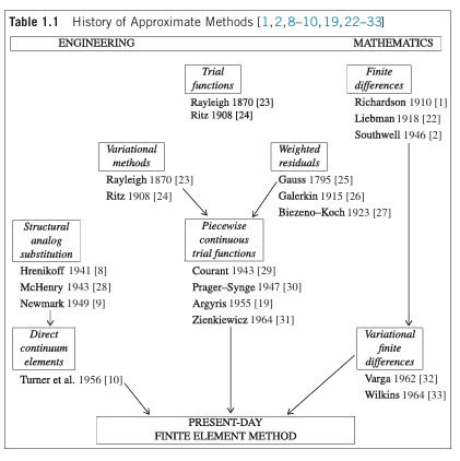
will give, in more detail, the mathematical basis which emerged from these classical ideas [1,22–27,29,30,32].
1.2 The structural element and the structural system
To introduce the reader to the general concept of discrete systems we shall first consider a structural engineering example with linear elastic behavior.
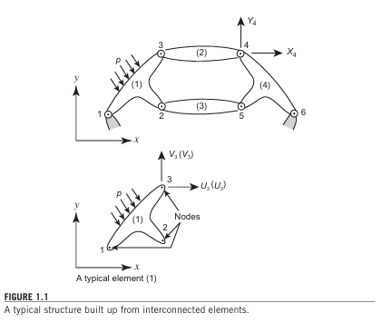
Figure1.1represents a two-dimensional structure assembled from individual com- ponents and interconnected at the nodes numbered 1 to 6. The joints at the nodes in this case are pinned so that moments cannot be trans mitted.
As a starting point it will be assumed that by separate calculation, or for that matter from the results of an experiment, the characteristics of each element are precisely known. Thus, if a typical element labeled (1) and associated with nodes 1, 2, and 3 is examined, the forces acting at the nodes are uniquely defined by the displacements of these nodes, the distributed loading acting on element (p), and its initial strain. The last may be due to temperature, shrinkage, or simply an initial “lack of fit.” The forces and the corresponding displacements are defined by appropriate components (U , V ) and (u, v) in a common coordinate system (x , y).
Listing the forces acting on all the nodes (three in the case illustrated) of element(1) as a matrix1 we have

and for the corresponding nodal displacements

Assuming linear elastic behavior of the element, the characteristic relationship will always be of the form

in which f1 represents the nodal forces required to balance any concentrated or dis- tributed loads acting on the element. The first of the terms represents the forces induced by displacement of the nodes. The matrix Ke is known as the stiffness matrix for element (e).
Equation (1.3) is illustrated by an example of an element with three nodes with the interconnection points capable of trans mitting only two components of force. Clearly, the same arguments and definitions will apply generally. Element (2) of the hypothetical structure will possess only two points of interconnection; others may have quite a large number of such points. Quite generally, therefore,
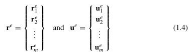
with each ra(e) and ua(e) possessing the same number of components or degrees offreedom.
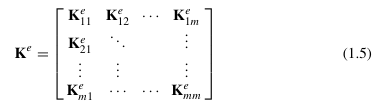
The stiffness matrices of the element will clearly always be square and of the form
1 A limited knowledge of matrix algebra will be assumed throughout this book. This is necessary for rea- sonable conciseness and forms a convenient bookkeeping form. For readers not familiar with the subject abrief appendix (Appendix A) is included in which sufficient principles of matrix algebra are given to fol- low the development intelligently. Matrices and vectors will be distinguished by bold print throughout.
in which K11(e) , K12(e), etc., are submatrices which are again square and of the size l × l ,
where l is the number of force and displacement components to be considered at each node. The element properties were assumed to follow a simple linear relationship. In principle, similar relationships could be established for nonlinear materials, but dis- cussion of such problems is not covered in this volume. Interested readers are referred to Ref. [37] for basic information on solid and structural mechanics applications and to Ref. [38] for applications to fluid dynamics problems. In most cases considered in this volume the element matrices Ke will be symmetric, that is

where (·)T denotes transpose of a matrix (see Appendix A).
更多内容见附件
免责声明:
本页面/内容部分素材来源于互联网公 开 信 息,旨在传递更多信息,不代表本平台立场。
版权归原作者或机构所有,如涉及侵权,请通过平台联系我们,我们将在核实后第一时间处理。
本平台对转载内容的真实性、准确性不作任何保证,用户需自行判断并承担使用风险。