东南大学齿轮箱振动数据集(含轴承、齿轮、复合故障)

2年前浏览10079

1 数据集描述

数据集可从https://github.com/cathysiyu/Mechanical-datasets/tree/master/dataset下载

实验平台如图1所示，主要由六个部分组成，分别是电机控制器、电机、行星齿轮箱、减速齿轮箱、负载以及负载控制器。共安装了七个型号为608A11振动传感器来分别采集行星齿轮箱和减速齿轮箱的x、y、z三轴以及电机z轴方向上的振动数据，采样频率为5120Hz。在该实验平台上，模拟并采集了不同工况下齿轮不同运行状态的振动数据，包括：断损、健康、缺齿、齿根裂纹以及齿轮表面磨损。

图1 实验平台实物图

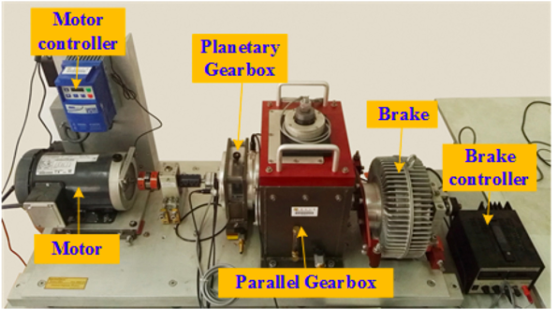
不同故障状态的齿轮都是提前委托加工好变转速可通过电机控制器来实现，而负载的变化则可以通过负载控制器实现。此外，故障齿轮安装在减速齿轮箱内，如图2所示。

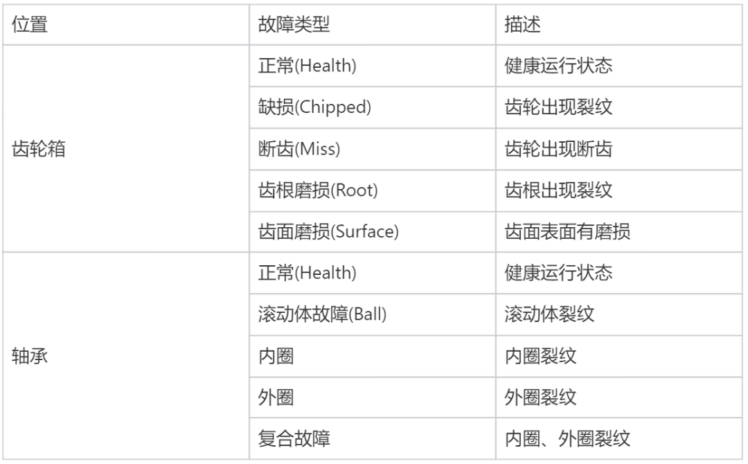
本数据集模拟了两种工况下的5种轴承运行状态和5种齿轮运行状态。两种工况分别为转速20Hz (1200rpm) -无负载0V (0Nm)与转速 30Hz (1800rpm) -有负载 2V (7.32Nm)。具体的故障类型描述如下表1所示。

哪个轴承、齿轮坏了信息未提供，轴承和齿轮尺寸参数也未提供。

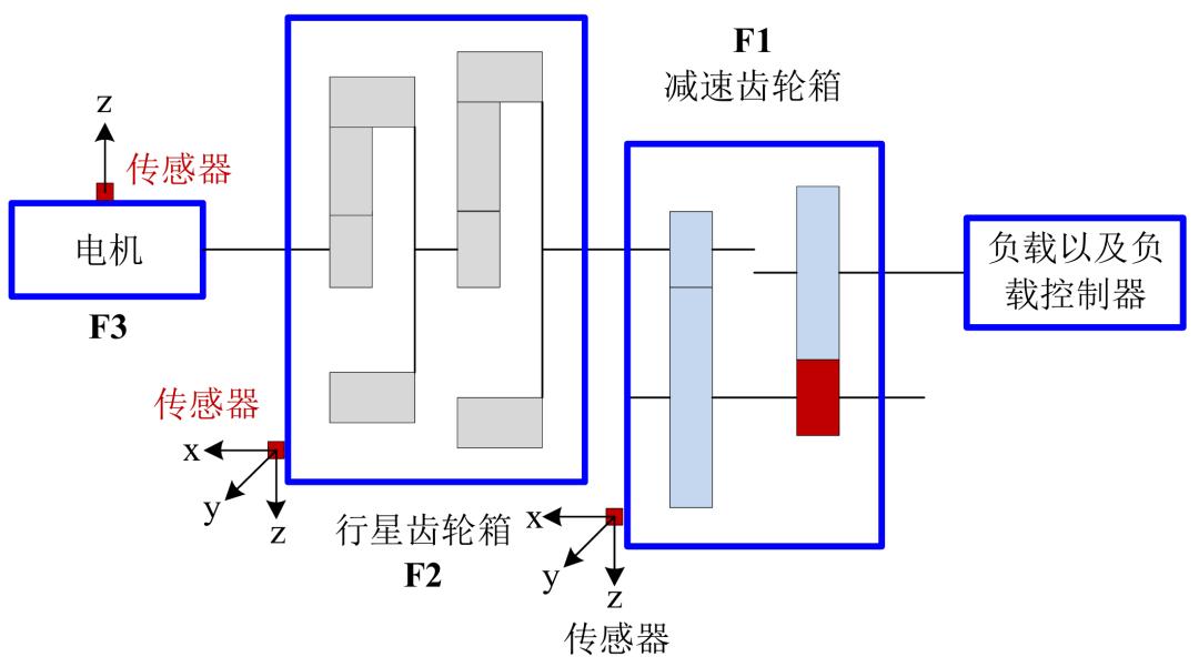
图2 实验平台的结构框图

表1 故障类型描述

2 时、频域分析

以下程序适合在jupyter notebook编辑器上运行。

2.1 导入包及函数

## 导入包from matplotlib import pyplot as pltfrom matplotlib import rcParamsimport numpy as npimport pandas as pdimport os
config = {    "font.family": 'serif', # 衬线字体    "font.size": 14, # 相当于小四大小    "font.serif": ['SimSun'], # 宋体    "mathtext.fontset": 'stix', # matplotlib渲染数学字体时使用的字体，和Times New Roman差别不大    'axes.unicode_minus': False # 处理负号，即-号}rcParams.update(config)

##========绘制时域信号图========##def plt_time_domain(arr, fs=1600, ylabel='Amp($m/s^2$)', title='原始数据时域图', img_save_path=None, x_vline=None, y_hline=None):    """    :fun: 绘制时域图模板    :param arr: 输入一维数组数据    :param fs: 采样频率    :param ylabel: y轴标签    :param title: 图标题    :return: None    """    import matplotlib.pyplot as plt    plt.rcParams['font.sans-serif'] = ['SimHei']  # 显示中文    plt.rcParams['axes.unicode_minus'] = False  # 显示负号    font = {'family': 'Times New Roman', 'size': '20', 'color': '0.5', 'weight': 'bold'}
    plt.figure(figsize=(12,4))    length = len(arr)    t = np.linspace(0, length/fs, length)    plt.plot(t, arr, c='g')    plt.xlabel('t(s)')    plt.ylabel(ylabel)    plt.title(title)    if x_vline:        plt.vlines(x=x_vline, ymin=np.min(arr), ymax=np.max(arr), linestyle='--', colors='r')    if y_hline:        plt.hlines(y=0.2, xmin=np.min(t), xmax=np.max(t), linestyle=':', colors='y')    #===保存图片====#    if img_save_path:        plt.savefig(img_save_path, dpi=500, bbox_inches = 'tight')    plt.show()

##========绘制频域信号图========##def plt_fft_img(arr, fs, ylabel='Amp(mg)', title='频域图', img_save_path=None, vline=None, hline=None, xlim=None):    """    :fun: 绘制频域图模板    :param arr: 输入一维时域数组数据    :param fs: 采样频率    :param ylabel: y轴标签    :param title: 图标题    :return: None    """    # 计算频域幅值    length = len(arr)    t = np.linspace(0, length/fs, length)    arr = arr - np.mean(arr)    fft_result = np.fft.fft(arr)    fft_freq= np.fft.fftfreq(len(arr), d=t[1]-t[0])  # FFT频率    fft_amp= 2*np.abs(fft_result)/len(t)                     # FFT幅值
    # 绘制频域图    plt.figure(figsize=(12,4))    plt.title(title)    plt.plot(fft_freq[0: int(len(t)/2)], fft_amp[0: int(len(t)/2)], label='Frequency Spectrum', color='b')    plt.xlabel('频率 (Hz)')    plt.ylabel('幅值')    plt.legend()    if vline:        plt.vlines(x=vline, ymin=np.min(fft_amp), ymax=np.max(fft_amp), linestyle='--', colors='r')    if hline:        plt.hlines(y=hline, xmin=np.min(fft_freq), xmax=np.max(fft_freq), linestyle=':', colors='y')    #===保存图片====#    if img_save_path:        plt.savefig(img_save_path, dpi=500, bbox_inches = 'tight')    if xlim: # 图片横坐标是否设置xlim        plt.xlim(0, xlim)      plt.tight_layout()    plt.show()

def plt_envelope_spectrum(data, fs, ylabel='Amp(mg)', title='包络谱图', img_save_path=None, vline=None, hline=None, xlim=None):    '''    fun: 绘制包络谱图    param data: 输入数据，1维array    param fs: 采样频率    param xlim: 图片横坐标xlim，default = None    param vline: 图片垂直线，default = None    '''    from scipy import fftpack    #=========做希尔伯特变换=======#    xt = data    ht = fftpack.hilbert(xt)    at = np.sqrt(xt**2+ht**2)   # 获得解析信号at = sqrt(xt^2 + ht^2)    at = at - np.mean(at)       # 去直流分量    fft_amp = np.fft.fft(at)         # 对解析信号at做fft变换获得幅值    fft_amp = np.abs(fft_amp)             # 对幅值求绝对值（此时的绝对值很大）    fft_amp = fft_amp/len(fft_amp)*2    fft_amp = fft_amp[0: int(len(fft_amp)/2)]  # 取正频率幅值    fft_freq = np.fft.fftfreq(len(at), d=1 / fs)  # 获取fft频率，此时包括正频率和负频率    fft_freq = fft_freq[0:int(len(fft_freq)/2)]  # 获取正频率    # 绘制包络谱图    plt.figure(figsize=(12,4))    plt.title(title)    plt.plot(fft_freq, fft_amp, color='b')    plt.xlabel('频率 (Hz)')    plt.ylabel('幅值')    if vline:        plt.vlines(x=vline, ymin=np.min(fft_amp), ymax=np.max(fft_amp), linestyle='--', colors='r')    if hline:        plt.hlines(y=hline, xmin=np.min(fft_freq), xmax=np.max(fft_freq), linestyle=':', colors='y')    #===保存图片====#    if img_save_path:        plt.savefig(img_save_path, dpi=500, bbox_inches = 'tight')    if xlim: # 图片横坐标是否设置xlim        plt.xlim(0, xlim)      plt.tight_layout()    plt.show()

2.2 轴承故障分析

2.2.1 读取数据

def data_read(file_path):    """    :fun: 读取csv数据    :param file_path: 文件路径    :return df:     """    try:        df = pd.read_csv(file_path, header=None)        df = df.iloc[16:, 0:8]        df = df.astype(float)    except:        df = pd.read_csv(file_path, header=None)        df.columns = ['acc_data']        df = df.iloc[16:,:]        # 首先，检查一下是否每个单元格都是字符串类型，如果不是，转换为字符串        df['acc_data'] = df['acc_data'].astype(str)
        # 使用str.split来分割列，参数expand=True表示分割后的结果将作为新的列添加到DataFrame中        df[['col1', 'col2', 'col3', 'col4', 'col5', 'col6', 'col7', 'col8', 'col9']] = df['acc_data'].str.split('\t', expand=True)        df = df[['col1', 'col2', 'col3', 'col4', 'col5', 'col6', 'col7', 'col8']]        df = df.astype(float)    return dffile_path = r'E:/03-公开数据集/东南大学数据集/gearbox/bearingset/ball_20_0.csv'df = data_read(file_path)acc_arr= df.iloc[:,7].valuesdf

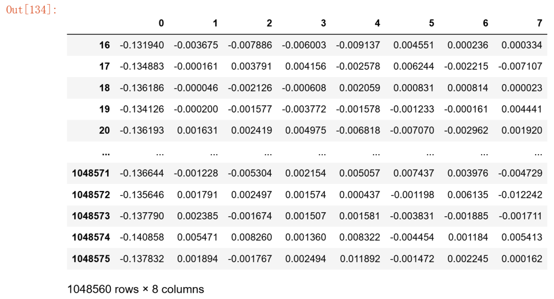
2.2.2 时域分析

fs = 5120##=======滚动体=====##file_path = r'E:/03-公开数据集/东南大学数据集/gearbox/bearingset/ball_20_0.csv'df = data_read(file_path)acc_arr= df.iloc[:,7].valuesfs = 5120file_name = r'ball_20_0.txt'plt_time_domain(acc_arr, fs=fs, title=file_name, img_save_path=time_img_save_path)kurtosis_value = calculate_kurtosis(acc_arr)print(f"Kurtosis of the signal: {kurtosis_value}")##=====外圈====##file_path = r'E:/03-公开数据集/东南大学数据集/gearbox/bearingset/outer_20_0.csv'df = data_read(file_path)acc_arr= df.iloc[:,7].valuesfile_name = r'outer_20_0.txt'plt_time_domain(acc_arr, fs=fs, title=file_name, img_save_path=time_img_save_path)kurtosis_value = calculate_kurtosis(acc_arr)print(f"Kurtosis of the signal: {kurtosis_value}")##=====内圈====##file_path = r'E:/03-公开数据集/东南大学数据集/gearbox/bearingset/inner_20_0.csv'df = data_read(file_path)acc_arr= df.iloc[:,7].valuesfile_name = r'inner_20_0.txt'plt_time_domain(acc_arr, fs=fs, title=file_name, img_save_path=time_img_save_path)kurtosis_value = calculate_kurtosis(acc_arr)print(f"Kurtosis of the signal: {kurtosis_value}")##=====复合====##file_path = r'E:/03-公开数据集/东南大学数据集/gearbox/bearingset/comb_20_0.csv'df = data_read(file_path)acc_arr= df.iloc[:,7].valuesfile_name = r'comb_20_0.txt'plt_time_domain(acc_arr, fs=fs, title=file_name, img_save_path=time_img_save_path)kurtosis_value = calculate_kurtosis(acc_arr[fs*15:])print(f"Kurtosis of the signal: {kurtosis_value}")##=====正常====##file_path = r'E:/03-公开数据集/东南大学数据集/gearbox/bearingset/health_20_0.csv'df = data_read(file_path)acc_arr= df.iloc[:,7].valuesfile_name = r'health_20_0.txt'plt_time_domain(acc_arr, fs=fs, title=file_name, img_save_path=time_img_save_path)kurtosis_value = calculate_kurtosis(acc_arr[fs*15:])print(f"Kurtosis of the signal: {kurtosis_value}")

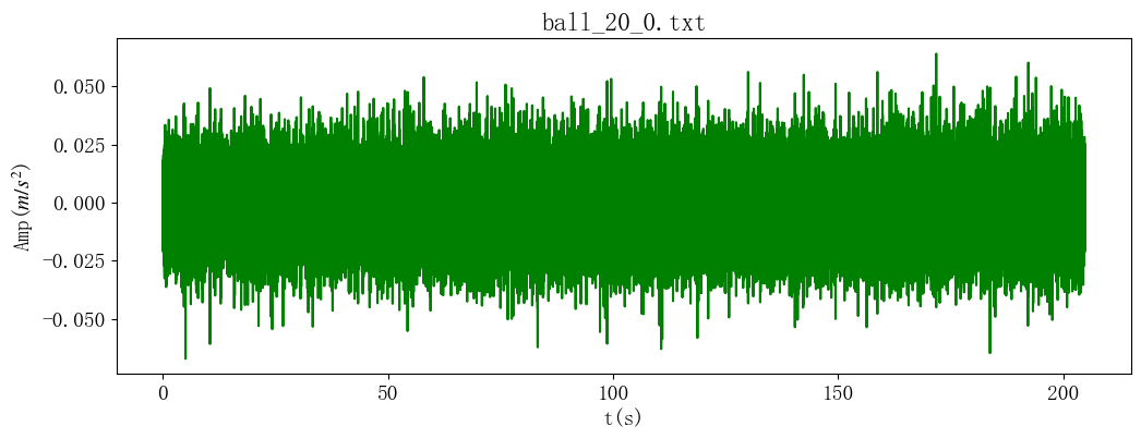
Kurtosis of the signal: 5.5406536985286845

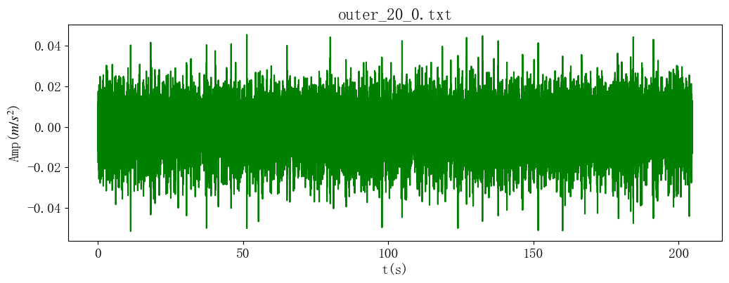
Kurtosis of the signal: 8.797642439965788

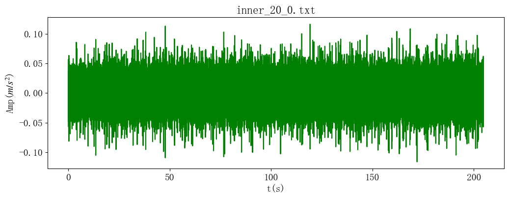
Kurtosis of the signal: 6.232998410057402

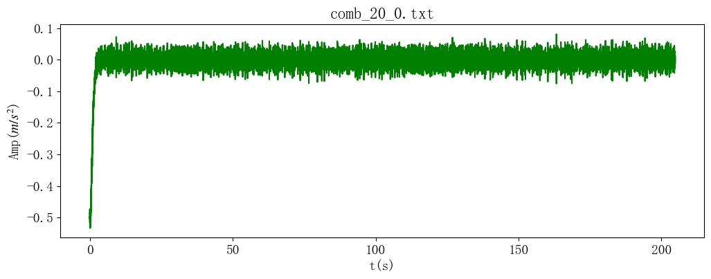
Kurtosis of the signal: 10.848358613561665

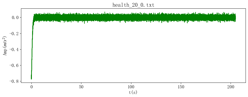
Kurtosis of the signal: 3.9275366437831924

分析：

峭度因子是一个能反映信号是否含有冲击信号的指标，正常状态峭度因子为3左右，当轴承有故障时，其峭度因子大于3；
从上述结果可知健康状态的峭度因子最小，为3.93，其它故障在5.5以上。

2.2.3 频域分析

fs = 5120##=======滚动体=====##file_path = r'E:/03-公开数据集/东南大学数据集/gearbox/bearingset/ball_20_0.csv'df = data_read(file_path)acc_arr= df.iloc[:,7].valuesfs = 5120file_name = r'ball_20_0.txt'plt_fft_img(acc_arr, fs=fs, title=file_name, img_save_path=fft_img_save_path, vline=[20, 40, 60, 80, 100], xlim=500)##=====外圈====##file_path = r'E:/03-公开数据集/东南大学数据集/gearbox/bearingset/outer_20_0.csv'df = data_read(file_path)acc_arr= df.iloc[:,7].valuesfile_name = r'outer_20_0.txt'plt_fft_img(acc_arr, fs=fs, title=file_name, img_save_path=fft_img_save_path, vline=[20, 40, 60, 80, 100], xlim=500)##=====内圈====##file_path = r'E:/03-公开数据集/东南大学数据集/gearbox/bearingset/inner_20_0.csv'df = data_read(file_path)acc_arr= df.iloc[:,7].valuesfile_name = r'inner_20_0.txt'plt_fft_img(acc_arr, fs=fs, title=file_name, img_save_path=fft_img_save_path, vline=[20, 40, 60, 80, 100], xlim=500)##=====复合====##file_path = r'E:/03-公开数据集/东南大学数据集/gearbox/bearingset/comb_20_0.csv'df = data_read(file_path)acc_arr= df.iloc[:,7].valuesfile_name = r'comb_20_0.txt'plt_fft_img(acc_arr, fs=fs, title=file_name, img_save_path=fft_img_save_path, vline=[20, 40, 60, 80, 100], xlim=500)##=====正常====##file_path = r'E:/03-公开数据集/东南大学数据集/gearbox/bearingset/health_20_0.csv'df = data_read(file_path)acc_arr= df.iloc[:,7].valuesfile_name = r'health_20_0.txt'plt_fft_img(acc_arr, fs=fs, title=file_name, img_save_path=fft_img_save_path, vline=[20, 40, 60, 80, 100], xlim=500)

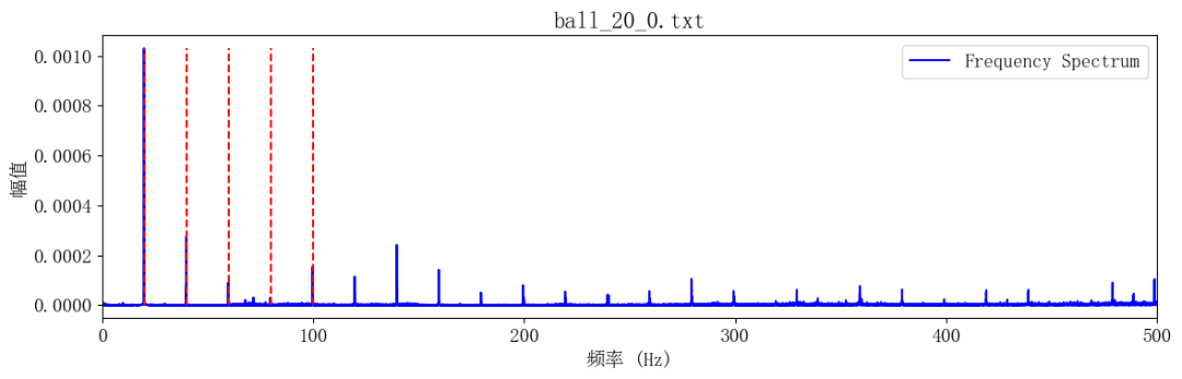
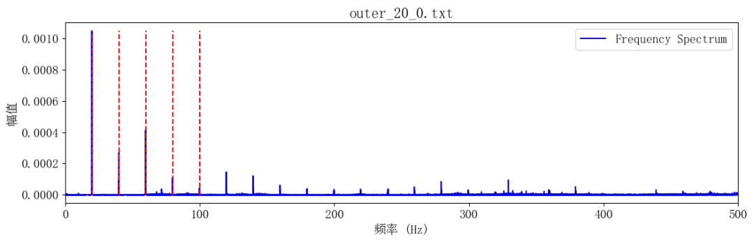
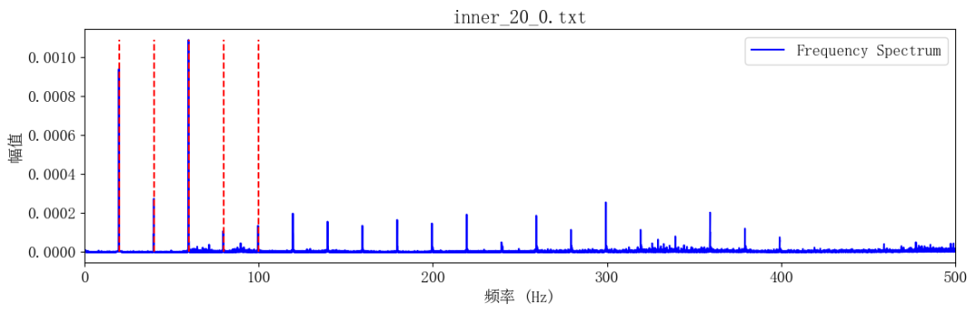
分析：

滚动体、外圈、内圈故障状态可以看到明显的转频及其倍频；
复合故障、正常状态可以看到明显的转频及其倍频。

2.2.4 包络谱分析

fs = 5120##=======滚动体=====##file_path = r'E:/03-公开数据集/东南大学数据集/gearbox/bearingset/ball_20_0.csv'df = data_read(file_path)acc_arr= df.iloc[:,7].valuesfs = 5120file_name = r'ball_20_0.txt'plt_envelope_spectrum(acc_arr, fs=fs, xlim=300, title=file_name)##=====外圈====##file_path = r'E:/03-公开数据集/东南大学数据集/gearbox/bearingset/outer_20_0.csv'df = data_read(file_path)acc_arr= df.iloc[:,7].valuesfile_name = r'outer_20_0.txt'plt_envelope_spectrum(acc_arr, fs=fs, xlim=300, title=file_name)##=====内圈====##file_path = r'E:/03-公开数据集/东南大学数据集/gearbox/bearingset/inner_20_0.csv'df = data_read(file_path)acc_arr= df.iloc[:,7].valuesfile_name = r'inner_20_0.txt'plt_envelope_spectrum(acc_arr, fs=fs, xlim=300, title=file_name)##=====复合====##file_path = r'E:/03-公开数据集/东南大学数据集/gearbox/bearingset/comb_20_0.csv'df = data_read(file_path)acc_arr= df.iloc[:,7].valuesfile_name = r'comb_20_0.txt'plt_envelope_spectrum(acc_arr, fs=fs, xlim=300, title=file_name)##=====正常====##file_path = r'E:/03-公开数据集/东南大学数据集/gearbox/bearingset/health_20_0.csv'df = data_read(file_path)acc_arr= df.iloc[:,7].valuesfile_name = r'health_20_0.txt'plt_envelope_spectrum(acc_arr, fs=fs, xlim=300, title=file_name)

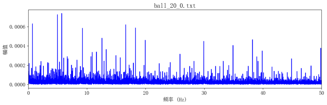
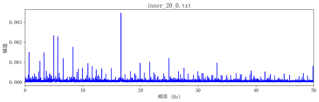
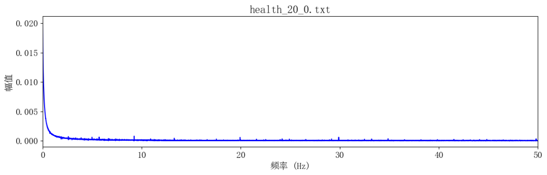
分析：

滚动体、外圈、内圈故障状态能看到突出峰值频率，但由于特征频率未知，不能判断是否对应上；
复合故障、正常状态没有看到明显的突出峰值频率。

2.3 齿轮故障分析

2.3.1 时域分析

fs = 5120##=======缺损=====##file_path = r'E:/03-公开数据集/东南大学数据集/gearbox/gearset/Chipped_20_0.csv'df = data_read(file_path)acc_arr= df.iloc[:,7].valuesfs = 5120file_name = r'Chipped_20_0.txt'plt_time_domain(acc_arr, fs=fs, title=file_name, img_save_path=time_img_save_path)kurtosis_value = calculate_kurtosis(acc_arr)print(f"Kurtosis of the signal: {kurtosis_value}")##=====断齿====##file_path = r'E:/03-公开数据集/东南大学数据集/gearbox/gearset/Miss_20_0.csv'df = data_read(file_path)acc_arr= df.iloc[:,7].valuesfile_name = r'Miss_20_0.txt'plt_time_domain(acc_arr, fs=fs, title=file_name, img_save_path=time_img_save_path)kurtosis_value = calculate_kurtosis(acc_arr)print(f"Kurtosis of the signal: {kurtosis_value}")##=====齿根磨损====##file_path = r'E:/03-公开数据集/东南大学数据集/gearbox/gearset/Root_20_0.csv'df = data_read(file_path)acc_arr= df.iloc[:,7].valuesfile_name = r'Root_20_0.txt'plt_time_domain(acc_arr, fs=fs, title=file_name, img_save_path=time_img_save_path)kurtosis_value = calculate_kurtosis(acc_arr)print(f"Kurtosis of the signal: {kurtosis_value}")##=====齿面磨损====##file_path = r'E:/03-公开数据集/东南大学数据集/gearbox/gearset/Surface_20_0.csv'df = data_read(file_path)acc_arr= df.iloc[:,7].valuesfile_name = r'Surface_20_0.txt'plt_time_domain(acc_arr, fs=fs, title=file_name, img_save_path=time_img_save_path)kurtosis_value = calculate_kurtosis(acc_arr)print(f"Kurtosis of the signal: {kurtosis_value}")##=====正常===##file_path = r'E:/03-公开数据集/东南大学数据集/gearbox/gearset/Health_20_0.csv'df = data_read(file_path)acc_arr= df.iloc[:,7].valuesfile_name = r'Health_20_0.txt'plt_time_domain(acc_arr, fs=fs, title=file_name, img_save_path=time_img_save_path)kurtosis_value = calculate_kurtosis(acc_arr)print(f"Kurtosis of the signal: {kurtosis_value}"

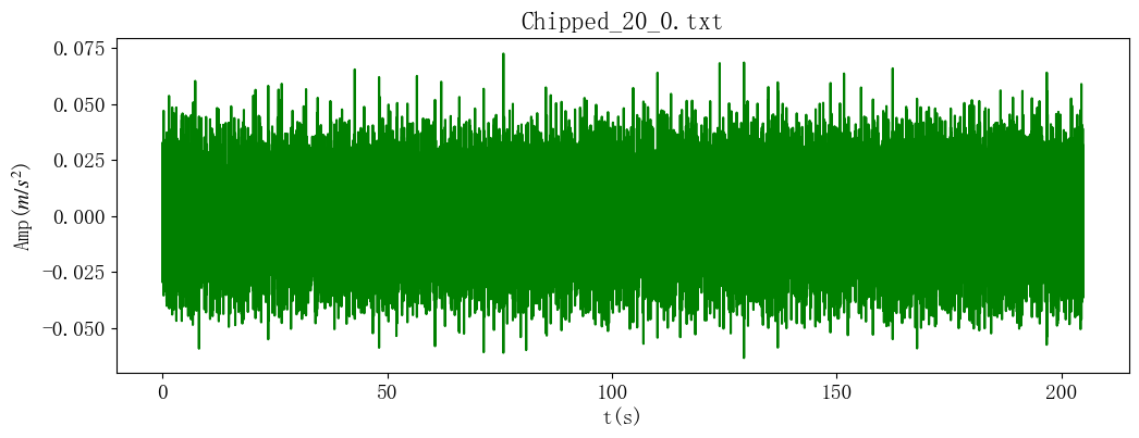
Kurtosis of the signal: 7.422209118627884

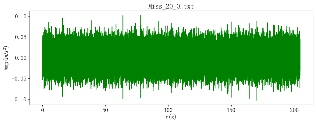
Kurtosis of the signal: 5.5002292494444

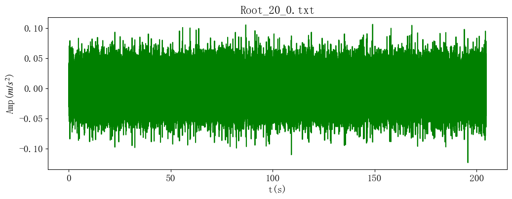
Kurtosis of the signal: 5.0213472682796505

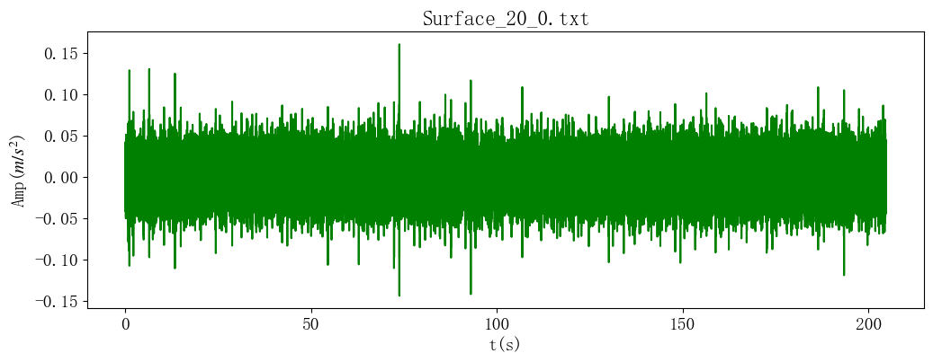
Kurtosis of the signal: 6.070086072663545

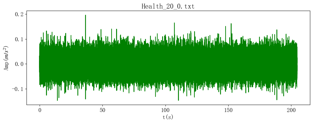
Kurtosis of the signal: 5.191029822842028

分析：

故障和正常齿轮的峭度因子均＞3，峭度因子对齿轮状态监测可能不太适用。

2.3.2 频域分析

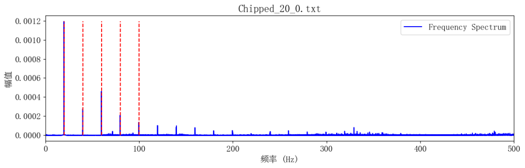
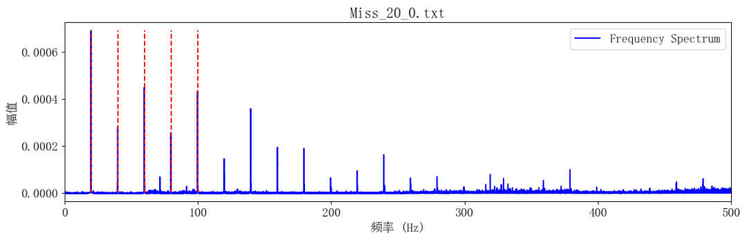
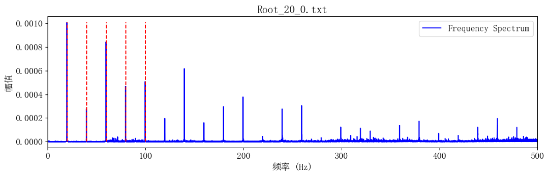
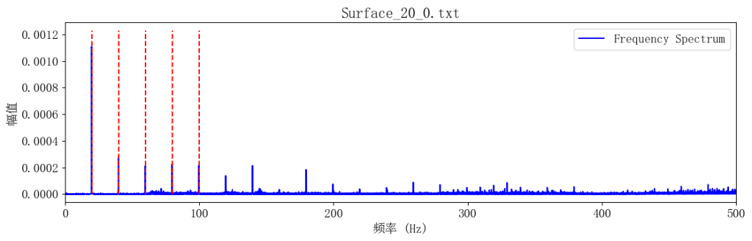
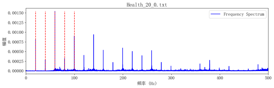
fs = 5120##=======缺损=====##file_path = r'E:/03-公开数据集/东南大学数据集/gearbox/gearset/Chipped_20_0.csv'df = data_read(file_path)acc_arr= df.iloc[:,7].valuesfs = 5120file_name = r'Chipped_20_0.txt'plt_fft_img(acc_arr, fs=fs, title=file_name, img_save_path=fft_img_save_path, vline=[20, 40, 60, 80, 100], xlim=500)##=====断齿====##file_path = r'E:/03-公开数据集/东南大学数据集/gearbox/gearset/Miss_20_0.csv'df = data_read(file_path)acc_arr= df.iloc[:,7].valuesfile_name = r'Miss_20_0.txt'plt_fft_img(acc_arr, fs=fs, title=file_name, img_save_path=fft_img_save_path, vline=[20, 40, 60, 80, 100], xlim=500)##=====齿根磨损====##file_path = r'E:/03-公开数据集/东南大学数据集/gearbox/gearset/Root_20_0.csv'df = data_read(file_path)acc_arr= df.iloc[:,7].valuesfile_name = r'Root_20_0.txt'plt_fft_img(acc_arr, fs=fs, title=file_name, img_save_path=fft_img_save_path, vline=[20, 40, 60, 80, 100], xlim=500)##=====齿面磨损====##file_path = r'E:/03-公开数据集/东南大学数据集/gearbox/gearset/Surface_20_0.csv'df = data_read(file_path)acc_arr= df.iloc[:,7].valuesfile_name = r'Surface_20_0.txt'plt_fft_img(acc_arr, fs=fs, title=file_name, img_save_path=fft_img_save_path, vline=[20, 40, 60, 80, 100], xlim=500)##=====正常===##file_path = r'E:/03-公开数据集/东南大学数据集/gearbox/gearset/Health_20_0.csv'df = data_read(file_path)acc_arr= df.iloc[:,7].valuesfile_name = r'Health_20_0.txt'plt_fft_img(acc_arr, fs=fs, title=file_name, img_save_path=fft_img_save_path, vline=[20, 40, 60, 80, 100], xlim=500)

file_path = r'E:/03-公开数据集/都灵理工大学变转速轴承数据集/都灵理工大学数据集/VariableSpeedAndLoad/C4A_400_496_1.mat'df = data_read(file_path)acc_arr= df['A1_x']plt_envelope_spectrum(acc_arr, fs=fs, xlim=3000, vline=[C_bsf, C_bsf*2])

分析：

故障和正常齿轮状态可以看到明显的转频及其倍频

2.3.3 包络谱分析

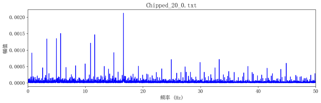
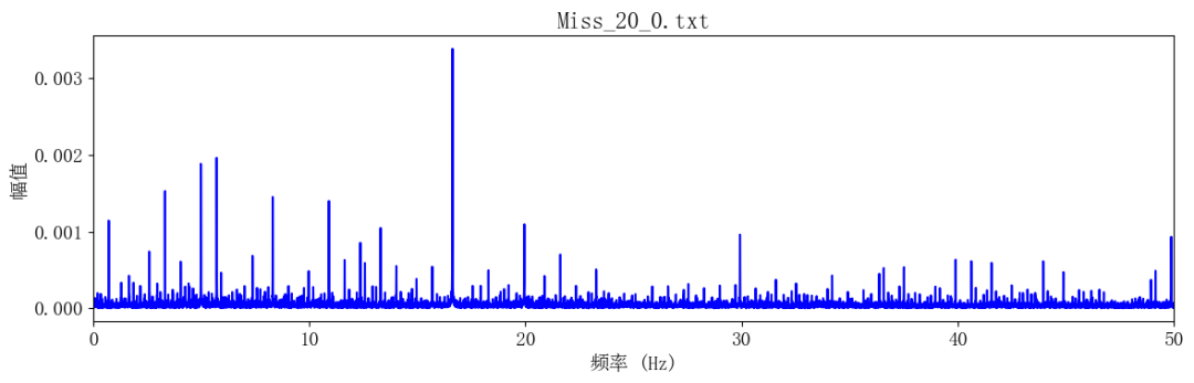
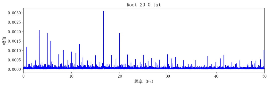
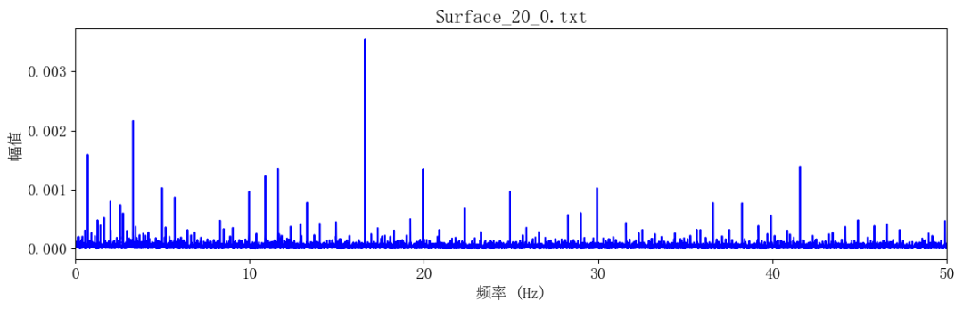
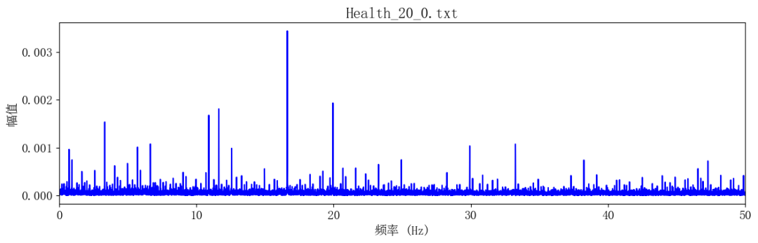
fs = 5120##=======缺损=====##file_path = r'E:/03-公开数据集/东南大学数据集/gearbox/gearset/Chipped_20_0.csv'df = data_read(file_path)acc_arr= df.iloc[:,7].valuesfile_name = r'Chipped_20_0.txt'plt_envelope_spectrum(acc_arr, fs=fs, xlim=300, title=file_name)##=====断齿====##file_path = r'E:/03-公开数据集/东南大学数据集/gearbox/gearset/Miss_20_0.csv'df = data_read(file_path)acc_arr= df.iloc[:,7].valuesfile_name = r'Miss_20_0.txt'plt_envelope_spectrum(acc_arr, fs=fs, xlim=300, title=file_name)##=====齿根磨损====##file_path = r'E:/03-公开数据集/东南大学数据集/gearbox/gearset/Root_20_0.csv'df = data_read(file_path)acc_arr= df.iloc[:,7].valuesfile_name = r'Root_20_0.txt'plt_envelope_spectrum(acc_arr, fs=fs, xlim=300, title=file_name)##=====齿面磨损====##file_path = r'E:/03-公开数据集/东南大学数据集/gearbox/gearset/Surface_20_0.csv'df = data_read(file_path)acc_arr= df.iloc[:,7].valuesfile_name = r'Surface_20_0.txt'plt_envelope_spectrum(acc_arr, fs=fs, xlim=300, title=file_name)##=====正常===##file_path = r'E:/03-公开数据集/东南大学数据集/gearbox/gearset/Health_20_0.csv'df = data_read(file_path)acc_arr= df.iloc[:,7].valuesfile_name = r'Health_20_0.txt'plt_envelope_spectrum(acc_arr, fs=fs, xlim=300, title=file_name

分析：

故障和正常齿轮状态可以看到明显的转频及其倍频，但由于特征频率未知，不能判断是否对应上。

参考文献：

[1] 陈超. 基于迁移学习的旋转机械故障诊断方法研究[D].东南大学,2022.

[2] 邵思羽.基于深度学习的旋转机械故障诊断方法研究[D].东南大学,2019.

[3] S. Shao, S. McAleer, R. Yan and P. Baldi, "Highly Accurate Machine Fault Diagnosis Using Deep Transfer Learning," in IEEE Transactions on Industrial Informatics, vol. 15, no. 4, pp. 2446-2455, April 2019, doi: 10.1109/TII.2018.2864759.

编辑：李正平

校核：陈凯歌、赵栓栓、董浩杰、曹希铭、赵学功、白亮、陈少华

该文资料搜集自网络，仅用作学术分享，不做商业用途，若侵权，后台联系小编进行删除

来源：故障诊断与python学习

XJTUGearbox和XJTUSuprgear齿轮箱振动数据集(含轴承、齿轮、变转速、复合故障)

目录1 数据集概述 1.1 声明 1.2 数据下载地址2 XJTUGearbox齿轮箱数据描述 2.1 实验设置 2.2 数据文件描述 2.3 XJTUGearbox实验台的技术资料3 XJTUSuprgear齿轮箱数据描述、 3.1 实验设置 3.2 数据文件描述 3.3 XJTUSuprgear实验台的技术资料4 绘制时域、频域、时频域图 4.1 XJTUGearbox数据集 4.1.1 数据读取 4.1.2 绘制时域图 4.1.3 绘制频域图 4.1.4 绘制时频域图 4.2 XJTUSuprgear数据集 4.2.1 数据读取 4.2.2 绘制时域图 4.2.3 绘制频域图 4.2.4 绘制时频域图 4.2.5 计算转速1 数据集概述1.1 声明XJTUGearbox和XJTuSuprgear数据集由中国陕西西安交通大学航空发动机研究所(http://iafe.xjtu.edu.cn/jgyjs/hkfdjyjs.htm)提供。这些故障诊断数据集是公开的，任何人都可以使用它们来验证诊断算法。出版物要求使用XJTUGearbox和xjtuupgear数据集引用以下论文。[1] Tianfu Li, Zheng Zhou, Sinan Li, Chuang Sun, Ruqiang Yan, Xuefeng Chen, “The emerging graphneural networks for intelligent fault diagnostics and prognostics: A guideline and a benchmark study,SignalProcessing,vol.168,pp.108653，2022.DOIMechanical Systems and10.1016/i.ymssp.2021.1086532 XJTUGearbox齿轮箱数据集描述2.1 实验设置实验平台如图1所示，由驱动电机、控制器、行星齿轮箱、平行齿轮箱和制动器组成。其中，电机类型是一个3相和3马力，其电源是三相交流电(230V，60/50Hz)。行星齿轮箱的X和Y方向安装了两个单轴加速度计(PCB352C04)来收集振动信号，并使用Y方向的信号。在实验中，在行星齿轮箱上模拟了4种行星轮故障和4种轴承故障。如图1(b)所示，齿轮失效包括齿面磨损、缺齿、齿根裂纹和断齿。轴承故障包括滚动体故障、内圈故障、外圈故障和上述三种轴承故障的混合故障。因此，与正常状态一起，共采集到9种振动信号。此外，在实验过程中电机转速设置为1800r/min，采样频率设置为20480Hz。 (a) 1.电机，2.控制器，3.行星齿轮箱，4.平行齿轮箱，5.制动器，6-7.水平和垂直方向的加速度计(b)齿轮和轴承的健康状况图1 XJTUGearbox数据集实验台 (a)实验台; (b)齿轮和轴承的健康状况2.2 数据文件描述如图2所示，XJTUGearbox数据集包括9个子文件夹。可以看出，行星齿轮箱的第一级行星轮是轴承故障，行星轮箱的第二级行星轮是齿轮故障。此外，每个子文件夹中包含2个txt文件，其中“Data_Chan1.txt”表示在Y方向收集的振动信号，“Data_Chan2.txt”表示在X方向收集的振动信号。2.3 XJTUGearbox试验台的技术资料XJTUGearbox试验台的技术信息如下图所示，详细信息可以在以下网址了解：https://spectraquest.com/drivetrains/details/dds/ 3 XJTUSuprgear齿轮箱数据集描述3.1 实验设置实验平台如图3(a)所示，其由驱动电机、皮带、轴和变速箱组成。其中，电机的型号为交流变频电机，其电源为单相交流(220V，60/50Hz)。12个单轴加速度计(PCB333B32)安装在变速箱上收集振动信号，并使用第一个传感器的信号。实验中，在直齿轮上加工了四种不同程度的裂纹，如图3(b)所示，再加上正常状态，共采集到五种振动信号。模拟了三种不同的转速，即900r/min、1200r/min，以及从0到1200r/min再到0的变转速。此外，在实验过程中，采样频率设置为10kHz。(a) 1.驱动电机，2.皮带，3.轴，4.加速度计，5.齿轮箱，6.负载，7.从动齿轮，8.主动齿轮(b) 直齿轮的健康状况图3 XJTUSuprgear数据集的测试台 (a)试验装置; (b)直齿轮的健康状况3.2 数据文件描述如图4所示，XJTUSuprgear数据集包括3个子文件夹，文件夹名称表示两个速度。此外，每个子文件夹包含5个txt文件，其中“suprgear02-15.txt“意味着试验齿轮的裂纹程度为0.2mm。此外，每个txt文件包含14列，其中第一列表示采集时间，最后一列表示速度脉冲信号，其他列表示由12个加速度计收集的振动信号。12个加速度计的详细安装位置如图5所示。图4 XJTUSuprgear数据集的内容图5 详细的传感器安装位置3.3 XJTUSuprgear实验台技术资料XJTUSuprgear试验台的技术信息如下所示：4 绘制时域、频域、时频域以下程序是基于jupyter notebook编辑器 4.1 XJTUGearbox数据集4.1.1 数据读取## 导入包from matplotlib import pyplot as pltfrom matplotlib import rcParamsimport numpy as npimport pandas as pdimport osconfig = { "font.family": 'serif', # 衬线字体 "font.size": 14, # 相当于小四大小 "font.serif": ['SimSun'], # 宋体 "mathtext.fontset": 'stix', # matplotlib渲染数学字体时使用的字体，和Times New Roman差别不大 'axes.unicode_minus': False # 处理负号，即-号}rcParams.update(config)##========绘制时域信号图========##def plt_time_domain(arr, fs=1600, ylabel='Amp($m/s^2$)', title='原始数据时域图', img_save_path=None, x_vline=None, y_hline=None): """ :fun: 绘制时域图模板 :param arr: 输入一维数组数据 :param fs: 采样频率 :param ylabel: y轴标签 :param title: 图标题 :return: None """ import matplotlib.pyplot as plt plt.rcParams['font.sans-serif'] = ['SimHei'] # 显示中文 plt.rcParams['axes.unicode_minus'] = False # 显示负号 font = {'family': 'Times New Roman', 'size': '20', 'color': '0.5', 'weight': 'bold'} plt.figure(figsize=(12,4)) length = len(arr) t = np.linspace(0, length/fs, length) plt.plot(t, arr, c='g') plt.xlabel('t(s)') plt.ylabel(ylabel) plt.title(title) if x_vline: plt.vlines(x=x_vline, ymin=np.min(arr), ymax=np.max(arr), linestyle='--', colors='r') if y_hline: plt.hlines(y=0.2, xmin=np.min(t), xmax=np.max(t), linestyle=':', colors='y') #===保存图片====# if img_save_path: plt.savefig(img_save_path, dpi=500, bbox_inches = 'tight') plt.show()##========绘制频域信号图========##def plt_fft_img(arr, fs, ylabel='Amp(mg)', title='频域图', img_save_path=None, vline=None, hline=None, xlim=None): """ :fun: 绘制频域图模板 :param arr: 输入一维时域数组数据 :param fs: 采样频率 :param ylabel: y轴标签 :param title: 图标题 :return: None """ # 计算频域幅值 length = len(arr) t = np.linspace(0, length/fs, length) arr = arr - np.mean(arr) fft_result = np.fft.fft(arr) fft_freq= np.fft.fftfreq(len(arr), d=t[1]-t[0]) # FFT频率 fft_amp= 2*np.abs(fft_result)/len(t) # FFT幅值 # 绘制频域图 plt.figure(figsize=(12,4)) plt.title(title) plt.plot(fft_freq[0: int(len(t)/2)], fft_amp[0: int(len(t)/2)], label='Frequency Spectrum', color='b') plt.xlabel('频率 (Hz)') plt.ylabel('幅值') plt.legend() if vline: plt.vlines(x=vline, ymin=np.min(fft_amp), ymax=np.max(fft_amp), linestyle='--', colors='r') if hline: plt.hlines(y=hline, xmin=np.min(fft_freq), xmax=np.max(fft_freq), linestyle=':', colors='y') #===保存图片====# if img_save_path: plt.savefig(img_save_path, dpi=500, bbox_inches = 'tight') if xlim: # 图片横坐标是否设置xlim plt.xlim(0, xlim) plt.tight_layout() plt.show()def plt_stft_img(arr, fs, ylabel='Amp(mg)', title='stft时频域图', img_save_path=None, vline=None, hline=None, xlim=None): """ :fun: 绘制stft时频域图模板 :param arr: 输入一维时域数组数据 :param fs: 采样频率 :param ylabel: y轴标签 :param title: 图标题 :return: None """ import scipy.signal as signal import numpy as np import matplotlib.pyplot as plt f, t, nd = signal.stft(arr, fs=fs, window='hann', nperseg=128, noverlap=64,nfft=None, detrend=False, return_onesided=True, boundary='odd', padded=False, axis=-1) # fs:时间序列的采样频率, nperseg:每个段的长度，默认为256(2^n) noverlap:段之间重叠的点数。如果没有则noverlap=nperseg/2 #window ：字符串或元组或数组，可选需要使用的窗。 # #如果window是一个字符串或元组，则传递给它window是数组类型，直接以其为窗，其长度必须是nperseg。 # 常用的窗函数有boxcar，triang，hamming， hann等，默认为Hann窗。 #nfft ：int，可选。如果需要零填充FFT，则为使用FFT的长度。如果为 None，则FFT长度为nperseg。默认为无 # detrend ：str或function或False，可选 # 指定如何去除每个段的趋势。如果类型参数传递给False，则不进行去除趋势。默认为False。 # return_onesided ：bool，可选 # 如果为True，则返回实际数据的单侧频谱。如果 False返回双侧频谱。默认为 True。请注意，对于复杂数据，始终返回双侧频谱。 # boundary ：str或None，可选 # 指定输入信号是否在两端扩展，以及如何生成新值，以使第一个窗口段在第一个输入点上居中。 # 这具有当所采用的窗函数从零开始时能够重建第一输入点的益处。 # 有效选项是['even', 'odd', 'constant', 'zeros', None]. # 默认为‘zeros’,对于补零操作[1, 2, 3, 4]变成[0, 1, 2, 3, 4, 0] 当nperseg=3. # padded：bool，可选 # 指定输入信号在末尾是否填充零以使信号精确地拟合为整数个窗口段，以便所有信号都包含在输出中。默认为True。 # 填充发生在边界扩展之后，如果边界不是None，则填充为True，默认情况下也是如此。 # axis ：int，可选 # 绘制STFT时频域图 plt.figure(figsize=(12,4)) plt.pcolormesh(t, f, np.abs(nd), vmin = np.min(np.abs(nd)), vmax = np.max(np.abs(nd))) plt.title(title) plt.xlabel('时间（t）') plt.ylabel('频率 (Hz)') if vline: plt.vlines(x=vline, ymin=np.min(fft_amp), ymax=np.max(fft_amp), linestyle='--', colors='r') if hline: plt.hlines(y=hline, xmin=np.min(fft_freq), xmax=np.max(fft_freq), linestyle=':', colors='y') #===保存图片====# if img_save_path: plt.savefig(img_save_path, dpi=500, bbox_inches = 'tight') if xlim: # 图片横坐标是否设置xlim plt.xlim(0, xlim) plt.tight_layout() plt.show()def data_read(file_path): """ :fun: 读取xls数据 :param file_path: 文件路径 :return df: """ df = pd.read_csv(file_path, header=None)[12:] # 第17行开始为加速度数据 df.columns = ['Acc_data'] df = df.astype(float) return dffile_path = r'E:/03-公开数据集/XJTUGearbox-and-XJTUSuprgear-datasets/XJTU_Gearbox/1ndBearing_ball/Data_Chan1.txt'df = data_read(file_path)acc_z_arr= df['Acc_data']df4.1.2 绘制时域图fs = 20480 # 采样频率file_name = r'1ndBearing_Ball.txt'##=====绘制时域数据====##time_img_save_path = file_path.replace('.txt', '时域_.png')plt_time_domain(acc_z_arr, fs=fs, title=file_name, img_save_path=time_img_save_path)4.1.3 绘制频域图fs = 20480file_name = r'1ndBearing_Ball.txt'##=====绘制频域数据====##fft_img_save_path = file_path.replace('.txt', '频域_.png')plt_fft_img(acc_z_arr, fs=fs, title=file_name, img_save_path=fft_img_save_path)4.1.3 绘制时频域图fs = 20480file_name = r'1ndBearing_Ball.txt'##=====绘制STFT时频域数据====##stft_img_save_path = file_path.replace('.txt', '时频域_.png') plt_stft_img(acc_z_arr, fs=fs, img_save_path=stft_img_save_path)4.2 XJTUSuprgear数据集4.2.1 数据读取def data_read(file_path): """ :fun: 读取xls数据 :param file_path: 文件路径 :return df: """ df = pd.read_csv(file_path, header = None) df.columns = ['Column'] # 使用 split 方法分割每行的单元格，expand=True 会将分割后的每个元素作为单独的列返回 df_split = df['Column'].str.split('\t', expand=True) # 将分割后的所有列转换为 float 类型 df_split = df_split.astype(float) # 重置索引，以便将分割后的列与原始 DataFrame 的索引对齐 df_split.reset_index(drop=True, inplace=True) return df_splitfile_path = r'E:/03-公开数据集/XJTUGearbox-and-XJTUSuprgear-datasets/XJTU_Spurgear/0-20-0Hz/spurgear10.txt'df = data_read(file_path)acc_z_arr = df.iloc[:,2].valuesdf4.2.2 绘制时域图fs = 10000file_name = r'spurgear10.txt'##=====绘制时域数据====##time_img_save_path = file_path.replace('.txt', '时域_.png')plt_time_domain(acc_z_arr, fs=fs, title=file_name, img_save_path=time_img_save_path)4.2.3 绘制频域图fs = 10000file_name = r'spurgear10.txt'##=====绘制频域数据====##fft_img_save_path = file_path.replace('.txt', '频域_.png')plt_fft_img(acc_z_arr, fs=fs, title=file_name, img_save_path=fft_img_save_path)4.2.4 绘制时频域图fs = 10000file_name = r'spurgear10.txt'##=====绘制STFT时频域数据====##stft_img_save_path = file_path.replace('.txt', '时频域_.png') plt_stft_img(acc_z_arr, fs=fs, img_save_path=stft_img_save_path)4.2.5 计算转速from scipy import signaldef tacho2rpm(x, fs, TLeveL=1, Slope=1, PPR=1, NewFs=None, Filter=13): time = len(x) x1 = np.arange(0, time, 1) t = x1 / fs xDiff = np.diff(np.sign(x - TLeveL).flatten()) tDiff = t[1:] NewFs = fs if Slope > 0: tTacho = tDiff[np.where(xDiff == 2)] else: tTacho = tDiff[np.where(xDiff == -2)] rpmt = 60 / (PPR * np.diff(tTacho)) rpmt = (rpmt[0:-1] + rpmt[1:]) / 2 tTacho = tTacho[1:-1] # 平滑处理 if Filter > 1: a = 1 b = 1 / Filter * np.ones((1, Filter)).flatten() rpmt = signal.filtfilt(b, a, rpmt) else: pass t = np.arange(0, t[-1] + 1 / NewFs, 1 / NewFs) rpm = np.interp(t, tTacho, rpmt) return t, rpmfile_path = r'E:/03-公开数据集/XJTUGearbox-and-XJTUSuprgear-datasets/XJTU_Spurgear/0-20-0Hz/spurgear06.txt'df = data_read(file_path)##======获取编码器信号时间======##tacho_arr = df.iloc[:,13].valuesfs = 10000length = len(tacho_arr)t = np.linspace(0, length/fs, length)plt.figure(figsize=[12,3])plt.plot(t, tacho_arr)plt.ylabel('幅值')plt.xlabel('时间(t)')plt.title('编码器信号图')##======将编码器信号计算得到转速信号====##t, rpm = tacho2rpm(tacho_arr, PPR=1, TLeveL=4, fs=fs)plt.figure(figsize=[12,3])plt.plot(t, rpm)plt.ylabel('转速(rpm)')plt.xlabel('时间(t)')plt.title('转速-时间图')plt.show()print('最大转速：', np.max(rpm))最大转速：1182.963277659338可见将编码器信号转换至转速后，转速最大为1183rpm，与实际1200rpm很接近。file_path = r'E:/03-公开数据集/XJTUGearbox-and-XJTUSuprgear-datasets/XJTU_Spurgear/15Hz/spurgear00.txt'df = data_read(file_path)##======获取编码器信号时间======##tacho_arr = df.iloc[:,13].valuesfs = 10000length = len(tacho_arr)t = np.linspace(0, length/fs, length)plt.figure(figsize=[12,3])plt.plot(t, tacho_arr)plt.ylabel('幅值')plt.xlabel('时间(t)')plt.title('编码器信号图')##======将编码器信号计算得到转速信号====##t, rpm = tacho2rpm(tacho_arr, PPR=1, TLeveL=4, fs=fs)plt.figure(figsize=[12,3])plt.plot(t, rpm)plt.ylabel('转速(rpm)')plt.xlabel('时间(t)')plt.title('转速-时间图(900rpm)')plt.show()可见将编码器信号转换至转速后，转速为884rpm，与实际900rpm很接近。file_path = r'E:/03-公开数据集/XJTUGearbox-and-XJTUSuprgear-datasets/XJTU_Spurgear/20Hz/spurgear00.txt'df = data_read(file_path)##======获取编码器信号时间======##tacho_arr = df.iloc[:,13].valuesfs = 10000length = len(tacho_arr)t = np.linspace(0, length/fs, length)plt.figure(figsize=[12,3])plt.plot(t, tacho_arr)plt.ylabel('幅值')plt.xlabel('时间(t)')plt.title('编码器信号图')##======将编码器信号计算得到转速信号====##t, rpm = tacho2rpm(tacho_arr, PPR=1, TLeveL=4, fs=fs)plt.figure(figsize=[12,3])plt.plot(t, rpm)plt.ylabel('转速(rpm)')plt.xlabel('时间(t)')plt.title('转速-时间图(1200rpm)')plt.show()可见将编码器信号转换至转速后，转速为1177rpm，与实际1200rpm很接近。参考资料：https://blog.csdn.net/m0_37262671/article/details/128727703(Python 信号处理——阶次分析(常规实现及另类实现))编辑：李正平校核：陈凯歌、赵栓栓、董浩杰、曹希铭、赵学功、白亮、陈少华该文资料搜集自网络，仅用作学术分享，不做商业用途，若侵权，后台联系小编进行删除来源：故障诊断与python学习

有附件