燃烧科学基础教程：从理论到工程应用（Peters_Summerschool_reference）

燃烧科学基础教程：从理论到工程应用（Peters_Summerschool_reference）

摘要：

本文是普林斯顿燃烧暑期学校讲义，系统梳理燃烧理论完整体系，从燃烧热力学、反应输运守恒方程切入，分预混、扩散火焰两大主线讲解层流燃烧基础。先推导组分分数、绝热火焰温度、化学平衡核心公式，给出 NASA 物性多项式与多组分物性参数；再建立反应流动质量、动量、能量守恒方程组，阐述输运定律与刘易斯数影响。基于单步渐近理论、甲烷四步简化机理分析预混火焰结构、层流火焰速度、拉伸与失稳机制；推导扩散火焰面模型、标量耗散率与熄火判据，涵盖对冲火焰、Tsuji 火焰、单液滴燃烧典型构型，同时介绍湍流燃烧基础框架，为 CFD 燃烧仿真、简化反应机理开发提供完备理论支撑。

Introduction

This text is a reduced English version of the material prepared for my combustion class at the RWTH Aachen Technical University.  It is intended as an introduction to the fundamentals of com- bustion science with the aim to supply the basic notions and equations for more detailed numerical investigations.  With modern computational tools and facilities numerical calculations with large codes aiming to predict the performance of combustion devices such as furnaces, reciprocative engines and gas turbines are feasible.  Whether they will partly or fully replace experimental in- vestigations will largely depend on the reliability of the combustion models used.  While there is a large scientific community concerned with Computational Fluid Dynamics and the improvement of turbulence models, the know-how in combustion modeling seems to be restricted to specialists. The reason for this is the complexity of the subject which requires advanced knowledge in thermo- dynamics, chemical kinetics and fluid mechanics. At the interface of these disciplines combustion emerges as a science which is able to predict rather than to merely describe experimentally ob- served phenomena.  In order to classify combustion phenomena it has been useful to introduce two types of situations with respect to mixing:  Premixed and non-premixed combustion.  For lami- nar flames issuing from a tube burner these two models of combustion are shown in Fig.  1. If fuel and air are already mixed within the tube, as in the case of a Bunsen burner, and the gas is ignited downstream, a premixed flame front will propagate towards the burner until it finds its steady state position in the form of the well-known Bunsen cone.  The fundamental quantity which describes this mode of combustion is the laminar burning velocity.  It is the velocity at which the flame front propagates normal to itself into the unburned mixture. For the steady state Bunsen cone the burn- ing velocity therefore must be equal to the flow velocity vn   normal to the flame front.  Behind the flame front yet unburnt intermediates as CO and H2  will mix with the air entrained from outside and lead to post flame oxidation and radiation. The other mode of combustion is that in a diffusion flame.  Here no air is mixed with the fuel within the tube of the burner.  This may be achieved but

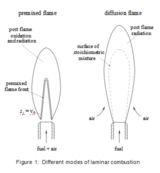
using a simply tube or by closing the air inlet in a Bunsen burner.  Then only fuel issues from the tube as shown in the second picture in Fig.  1.  It mixes with the surrounding air by convection and diffusion during combustion. Optimal conditions for combustion are restricted to the vicinity of the surface of stoichiometric mixture. This is the surface where fuel and air are locally mixed in a proportion that allows both to be entirely consumed.  This will lead to the highest flame tempera- ture and, due to the temperature sensitivity of the chemical reactions, to the fastest reaction rates. Since in most cases combustion is much faster than diffusion the latter is the rate limiting step that controls the entire process. This is the reason why those flames, where the reactants are initially non-premixed, are called diffusion flames.  Premixed flames appear with a blue to bluish-green color, while diffusion flames radiate in a bright yellow color.  The blue color of premixed flames is due to chemiluminescence of some excited species (C2  and CH radicals), while the yellow color of diffusion flames is caused by radiating soot particles which dominate over the chemiluminescence that is also present in at the base of a diffusion flame. Close to the burner there appears blue layer since the local residence time is too short for soot particles to be formed. This leads to the conclu- sion that the color of a flame is characteristic for the available residence time rather than the mode  of mixing.   Premixed Flames are used whenever intense combustion is required within a small volume. This is the case in household appliances and spark ignition engines.  In such an engine a premixed turbulent flame front propagates from the spark through the combustion chamber until the entire mixture is burnt. An example for non-premixed combustion are Diesel engines, where a liquid fuel spray is injected into the compressed hot air within the cylinder.  It rapidly evaporates and mixes with the air and then auto-ignition under partly premixed conditions.  The final stage at combustion occurs under non-premixed conditions.  Finally, large combustion devices such as furnaces, operate under non-premixed conditions because premixing of large volumes of fuel and air would represent a serious safety hazard.

The classification of combustion phenomena into premixed and non-premixed combustion is used throughout this text. After an introduction into the basic thermodynamics of combustion sys- tems in Lecture 1, a simplified calculation of the adiabatic flame temperature and an approximate calculation of equilibrium constants is presented in Lecture 2.  The balance equations of fluid dy- namics are presented shortly in Lecture 3, laminar premixed flames are treated in Lecture 4-7 and laminar diffusion flames in Lectures 8 and 9.  Then an introduction into turbulent combustion is given in Lecture 10.  Premixed turbulent combustion is presented in terms of the regime diagram in Lecture 11, the level set approach and the turbulent burning velocity is presented in Lectures 12 and 13, while non-premixed turbulent combustion is treated in Lecture 14.  Finally, in Lecture 15 applications in engines closes the text.  In preparing these lectures and the text I have enjoyed the support from many of my students and friends. I am particular indebted to Bernd Binninger for cross-reading the manuscript and for the preparation of many of the figures.  I could also rely on the efficiency of Sonja Engels in preparing the manuscript.

Lecture 1  Thermodynamics of Combustion Systems

Combustion is a mass and energy conversion process during which chemical bond energy is transformed to thermal energy.  The fuel reacts with the oxygen of the air to form products such as carbon dioxide and water which have a lower enthalpy of formation or reference enthalpy than the reactants. The details of the reaction mechanism that leads from the reactants to the products will be presented by other lectures of this summer school.  In this lecture we will only consider the initial and the final state of a homogeneous system and use the classical balance laws of thermodynamics. This global view is much simpler and leads in Lecture 2 to some useful results such as the adiabatic flame temperature.  We will first present definitions of concentrations and other thermodynamic variables and present the mass and energy balance for multicomponent systems.

1.1   Mole Fractions and Mass Fractions

When chemical species react with each other to form other species, their basic constituents, the chemical elements are conserved.  The particular atom defining the element, a C atom within a CH4  molecule, for example, will be found within the CO2  molecule after combustion is completed. In order to describe the chemical transformation between species quantitatively, we need to intro- duce definitions for concentrations. Since different descriptions are being used in the combustion  literature, it is useful to present these first and to relate them to each other.

1.2   The Mole Fraction

We consider a multi-component system with k different chemical species that contains a large number of molecules. Then 6.0236·1023 molecules are defined as one mole. The number of moles of species i denoted by ni  and its sum is the total number of moles ns

The mole fraction of species i is now defined

1.2.1   The Mass Fraction

The mass mi  of all molecules of species i is related to its number of moles by

where Wi  is the molecular weight of species i.  For some important species in combustion Wi   is given in Tab. 2.1. The total mass of all molecules in the mixture is

The mass fraction of species i is now defined

Defining the mean molecular weight W by

one obtains the relation between mole fractions and mass fractions as

The mean molecular weight may be calculated if either the mole fractions or the mass fractions

are known

1.2.2   The Mass Fraction of Elements

In addition, the mass fraction of elements is very useful in combustion.  While the mass of the species changes due to chemical reactions, the mass of the elements is conserved.  We denote by mj  the mass of all atoms of element j contained in all molecules of the system.  If aij   is the number of atoms of element j  in a molecule of species i and Wj   is the molecular weight of that atom, the mass of all atoms j in the system is

where ke  is the total number of elements in the system. The mass fraction of element j is then

Notice that no meaningful definition for the mole fraction of elements can be given because only the mass of the elements is conserved. From the definitions above it follows that

1.2.3   The Partial Molar Density

An additional variable defining a concentration, that is frequently used in chemical kinetics, is the number of moles per unit volume or partial molar density

where V is the volume of the system. The molar density of the system is then

1.2.4   The Partial Density

The density and the partial density are defined

The partial molar density is related to the partial density and the mass fraction by

原资料见附件

免责声明：

本页面/内容部分素材来源于互联网公 开 信 息，旨在传递更多信息，不代表本平台立场。

版权归原作者或机构所有，如涉及侵权，请通过平台联系我们，我们将在核实后第一时间处理。

本平台对转载内容的真实性、准确性不作任何保证，用户需自行判断并承担使用风险。