工程师流体力学（研究生教材）Fluid mechanics for engineers

工程师流体力学（研究生教材）Fluid mechanics for engineers

摘要：

本文为面向研究生的工程流体力学教材第五章积分守恒律内容，依托雷诺输运定理推导流体质量、线动量、角动量、能量四大积分守恒方程。结合控制体积法建立适用于叶轮机械、喷管、燃烧室等工程部件的求解模型，引入总焓、熵增与总压损失理论，分析不可逆流动损耗。系统推导涡轮、压气机级欧拉方程，定义流量系数、负荷系数、反应度等无量纲级参数，结合自由涡径向平衡理论阐述叶片展向流动分布，完整给出叶轮机械能量转换统一分析框架，为热力叶轮气动设计、性能评估提供基础理论工具。

Preface

The contents of this book covers the material required in the Fluid Mechanics Graduate Core Course (MEEN-621) and in Advanced Fluid Mechanics, a Ph.D-level elective course  (MEEN-622), both of which I have been teaching at Texas A&M University for the past two decades. While there are numerous undergraduate fluid mechanics texts on the market for engineering students and instructors to choose from, there are only limited texts that comprehensively address the particular needs of graduate  engineering  fluid  mechanics  courses.  To  complement  the  lecture materials, the instructors more often recommend several texts, each of which treats special topics of fluid mechanics. This circumstance and the need to have a textbook that covers the materials needed in the above courses gave the impetus to provide the graduate engineering community with a coherent textbook that comprehensively addresses their needs for an advanced fluid mechanics text. Although this text book is primarily aimed at   mechanical engineering students, it is equally suitable for aerospace engineering, civil engineering, other engineering disciplines, and especially those practicing professionals who perform CFD-simulation on a routine basis and would like to know more about the underlying physics of the commercial codes they use. Furthermore, it is suitable for self study, provided that the reader has a sufficient knowledge of calculus and differential equations.

In the past, because of the lack of advanced computational capability, the subject of fluid  mechanics  was  artificially  subdivided  into  inviscid,  viscous  (laminar, turbulent), incompressible, compressible, subsonic, supersonic and hypersonic flows. With today’s state of computation, there is no need for this subdivision. The motion of a fluid is accurately described by the Navier-Stokes equations. These equations require  modeling of the relationship between the stress and deformation tensor for linear and nonlinear fluids only. Efforts by many researchers around the globe are aimed at directly solving the Navier-Stokes equations (DNS) without introducing the Reynolds stress tensor, which is the result of an artificial decomposition of the velocity field into a mean and fluctuating part. The use of DNS for engineering applications seems to be out of reach because the computation time and resources required to perform a DNS-calculation are excessive at this time. Considering this constraining circumstance, engineers have to resort to Navier-Stokes solvers that are based on Reynolds decomposition. It requires modeling of the transition process and the Reynolds stress tensor to which three chapters ofthis book are dedicated.

The book is structured in such a way that all conservation laws, their derivatives and related equations are written in coordinate invariant forms. This type of structure enables the reader to use Cartesian, orthogonal curvilinear, or non-orthogonal body fitted coordinate systems. The coordinate invariant equations are then  decomposed  into components by utilizing the index notation of the corresponding coordinate systems.  The  use   of  a   coordinate  invariant   form  is  particularly   essential  in understanding the underlying physics of the turbulence, its implementation into the Navier-Stokes equations, and the necessary mathematical manipulations to arrive at different correlations. The resulting correlations are the basis for the following turbulence modeling. It is worth noting that in standard textbooks of turbulence, index notations are used throughout with almost no explanation of how they were brought about.  This  circumstance  adds  to  the  difficulty  in understanding  the nature  of turbulence by readers who are freshly exposed to the problematics of turbulence. Introducing the coordinate invariant approach makes it easier for the reader to follow step-by-step  mathematical  manipulations,  arrive  at  the  index  notation  and  the component decomposition. This, however, requires the knowledge of tensor an alysis. Chapter 2 gives a concise overview of the tensor an alysis essential for describing the conservation laws in coordinate invariant form, how to accomplish the index notation, and the component decomposition into different coordinate systems.

Using the tensor ana lytical knowledge gained from Chapter 2, it is rigorously applied to the following chapters. In Chapter 3, that deals with the kinematics offlow motion, the Jacobian transformation describes in detail how a time dependent volume integral is treated. In Chapter 4 and 5 conservation laws of fluid mechanics and thermodynamics are treated in differential and integral forms. These chapters are the basis for what follows in Chapters 7, 8, 9, 10 and 11 which exclusively deal with viscous flows. Before discussing the latter, the special case of inviscid flows is presented where the order of magnitude of a viscosity force compared with the convective forces are neglected. The potential flow, a special case of inviscid flow characterized by zero vorticity  v -  0 , exhibited a major topic in fluid mechanics in pre-CFD era. In recent years, however, its relevance has been diminished. Despite this fact, I presented it in this book for two reasons. (1) Despite its major short comings to describe the flow pattern directly close to the surface, because it does not satisfy the no-slip condition, it reflects a reasonably good picture of the flow outside the boundary layer. (2) Combined with the boundary layer calculation procedure, it helps acquiring a reasonably accurate picture of the flow field outside and inside the boundary  layer.  This,  of course,  is  valid  as  long  as the boundary  layer  is not separated. For calculating the potential flows, conformal transformation is used where the necessary basics are presented in Chapter 6, which is concluded by discussing different vorticity theorems.

Particular issues of laminar flow at different pressure gradients associated with the flow separation in conjunction with the wall curvature constitute the content of Chapter 7 which seamlessly merges into Chapter 8 that starts with the stability of laminar, followed by laminar-turbulent transition, intermittency function and its implementation  into Navier-Stokes.  Averaging  the Navier-Stokes  equation  that includes the intermittency function leading to the Reynolds averaged Navier-Stokes equation (RANS), concludes Chapter 8. In discussing the RANS-equations, two quantities have to be accurately modeled. One is the intermittency function, and the other is the Reynolds stress tensor with its nine components. Inaccurate modeling of these two quantities leads to a multiplicative error of their product. The transition was already discussed in Chapter 8 but the Reynolds stress tensor remains to be modeled.

This, however, requires the knowledge  and understanding  of turbulence before attempts are made to model it. In Chapter 9, I tried to present the quintessence of turbulence required  for  a  graduate  level mechanical  engineering  course  and to critically discuss several different models. While Chapter 9 predominantly deals with the wall turbulence, Chapter 10 treats different aspects of free turbulent flows and their general relevance in engineering. Among different free turbulent flows, the process of development and decay of wakes under positive, zero, and negative pressure  gradients  is  of particular  engineering  relevance.  With  the  aid  of  the characteristics developed in Chapter 10, this process of wake development and decay can be described accurately.

Chapter  11 is  entirely dedicated to the physics of laminar, transitional and turbulent  boundary  layers.  This  topic  has  been  of  particular  relevance  to  the engineering community. It is treated in integral and differential forms and applied to laminar, transitional, turbulent boundary layers, and heat transfer.

Chapter 12 deals with the compressible flow. At first glance, this topic seems to be dissonant with the rest ofthe book. Despite this, I decided to integrate it into this book for two reasons: (1) Due to a complete change of the flow pattern from subsonic to supersonic, associated with a system of oblique shocks makes it imperative to present this topic in an advanced engineering fluid text; (2) Unsteady compressible flow with moving shockwaves occurs frequently in many engines such as transonic turbines and compressors, operating in off-design and even design conditions. A simple example is the shock tube, where the shock front hits the one end of the tube to be reflected to the other end. A set of steady state conservation laws does not describe this unsteady phenomenon. An entire set ofunsteady differential equations must be called upon which is presented in Chapter 12. Arriving at this point, the students need to know the basics of gas dynamics. I had two options, either refer the reader to existing gas dynamics textbooks, or present a concise account of what is most essential in following this chapter. I decided on the second option.

At the end of each chapter, there is a section that entails problems and projects. In selecting the problems, I carefully selected those from the book Fluid Mechanics Problems and Solutions by Professor Spurk of Technische Universität Darmstadt which I translated in 1997. This book contains a number of highly advanced problems followed by  very  detailed  solutions.  I  strongly  recommend  this  book  to  those instructors who are in charge of teaching graduate fluid mechanics as a source of advanced problems. My sincere thanks goto Professor Spurk, my former Co-Advisor, for giving me the permission . Besides the problems, a number of demanding projects are presented that are aimed at getting the readers involved in solving CFD-type of problems. In the course of teaching the advanced Fluid Mechanics course MEEN- 622, I insist that the students present the project solution in the form of a technical paper in the format required by ASME Transactions, Journal of Fluid Engineering.

In typing several thousand equations, errors may occur. I tried hard to eliminate typing, spelling  and other errors, but I have no doubt that some remain to be found by readers. In this case, I sincerely appreciate the reader notifying me of any mistakes found; the electronic address is given below. I also welcome any comments or suggestions regarding the improvement of future editions ofthe book.

My sincere thanks are due to many fine individuals and institutions. First and foremost, I would like to thank the faculty of the Technische Universität Darmstadt from whom I received my entire engineering education. I finalized major chapters of the manuscript during my sabbatical in Germany where I received the Alexander von Humboldt Prize. I am indebted to the Alexander von Humboldt Foundation for this Prize and the material support for my research sabbatical in Germany. My thanks are extended to Professor Bernd Stoffel, Professor Ditmar Hennecke, and Dipl. Ing. Bernd Matyschok for providing me with a very congenial working environment.

I  am  also  indebted  to  TAMU  administration  for  partially  supporting  my sabbatical which helped me in finalizing the book. Special thanks are due to Mrs. Mahalia Nix who helped me in cross-referencing the equations and figures and rendered other editorial assistance.

Last, but not least, my special thanks go to my family, Susan and Wilfried for their support throughout this endeavor.

M.T. Schobeiri

August 2009

College Station, Texas

tschobeiri@mengr.tamu.edu

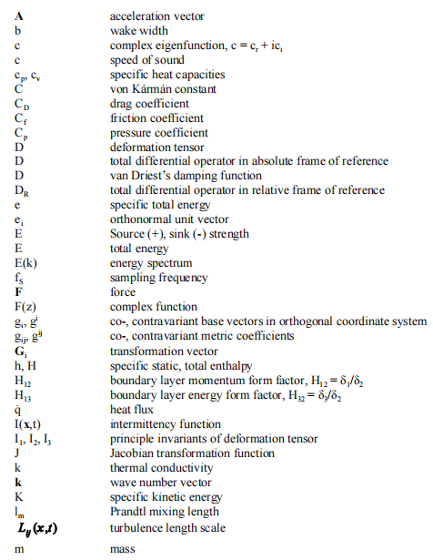
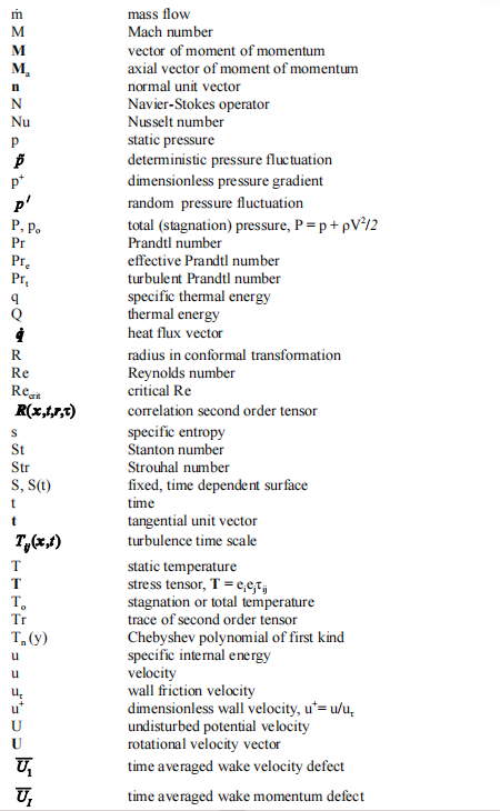
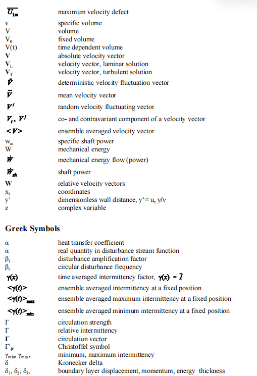
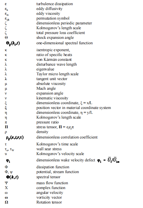
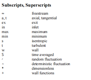
Nomenclature

1    Introduction

The structure of thermo-fluid sciences rests on three pillars, namely fluid mechanics, thermodynamics, and heat transfer. While fluid mechanics’ principles are involved in  open  system  thermodynamics  processes,  they  play  a  primary  role  in  every convective heat transfer problem. Fluid mechanics deals with the motion of fluid particles and describe their behavior under any dynamic condition where the particle velocity may range from low subsonic to hypersonic. It also includes the special case termed fluid statics, where the fluid velocity approaches zero. Fluids are encountered in  various  forms  including  homogeneous   liquids,  unsaturated,   saturated,  and superheated vapors, polymers and inhomogeneous liquids and gases. As we will see in the following chapters, only a few equations govern the motion of a fluid that consists of molecules. At microscopic level, the molecules continuously interact with each other moving with random velocities. The degree of interaction and the mutual exchange of momentum between the molecules increases with increasing temperature, thus, contributing to an intensive and random molecular motion.

1.1 Continuum Hypothesis

The random motion mentioned above, however, does not allow to define a molecular velocity at a fixed spatial position. To circumvent this dilemma, particularly for gases, we consider the mass contained in a volume element vG which has the same order of magnitude as the volume spanned by the mean free path of the gas molecules. The volume VG has a comparable order of magnitude for a molecule of a liquid V .

Thus, a fluid can be treated as a continuum if the volume 8VG occupied by the mass does not experience excessive changes. This implies that the ratio

does not depend upon the volume vG . This is known as the continuum hypothesis that holds for systems, whose dimensions are much larger than the mean free path of the molecules. Accepting this hypothesis, one may think of a fluid particle as a collection of molecules that moves with a velocity that is equal to the average velocity of all molecules that are contained in the fluid particle. With this assumption, the density defined in Eq. (1.1) is considered as a point function that can be dealt with as a thermodynamic property of the system. If thep-v-T-behavior of a fluid is given, the density at any position vector x and time  t can immediately be determined by

providing an information about two other thermodynamic properties. For fluids that   are frequently used in technical applications, the p-v-T behavior is available from experiments in the form of p-v, h-s, or T-s tables or diagrams. For computational purposes, the experimental points are fitted with a series of algebraic equations that allow  a  quick  determination  of density  by  using  two  arbitrary  thermodynamic properties.

1.2 Molecular Viscosity

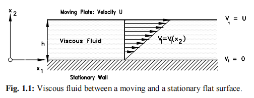
Molecular viscosity is the fluid property that causes friction. Fig. 1.1 gives a clear physical picture of the friction in a viscous fluid. A flat plate placed at the top of a particular viscous fluid is moving with a uniform velocity  vi  -  U relative to the stationary bottom wall.

The following observations were made during experimentation:

1) In order to move the plate, a certain force  F1 must be exerted in x1-direction.

2) The fluid sticks to the plate surface that moves with the velocity U.

3) The velocity difference between the stationary bottom wall and the moving top wall causes a velocity change which is, in this particular case, linear.

4) The force F1  is directly proportional to the velocity change and the area of the plate.

These observations lead to the conclusion that one may set:

Multiplying the proportionality (1.2) by a factor μ which is the  substance property viscosity, results in an equation for the friction force in x1-direction:

The subsequent division of Eq. (1.3) by the plate area A gives the shear stress component τ21 :

Equation (1.4) is the Newton’s equation of viscosity for this particular case. The first subscript refers to the plane perpendicular to the x2-coordinate; the second refers to the direction of shear stress. Equation (1.4) is valid for a two-dimensional flow of a particular  class  of fluids,  the Newtonian Fluids, whose  shear  stress  is  linearly proportional to the velocity change. The general three-dimensional version derived and discussed in Chapter 4 is:

with D as the deformation tensor. The coefficient λ is given by       , with μ as the absolute viscosity and  the bulk viscosity. Inserting Eq. (1.5) into the equation of motion (see Chapter 4), the resulting equation independently developed by Navier [ 1] and Stokes [2] completely describes the motion of a viscous fluid. In a coordinate invariant form the Navier-Stokes equation reads:

Although Eq. (1.6) has been known since the publication of the famous paper by Navier in 1823, with the exception of few special cases, it was not possible to find solutions for cases of practical interests. Neglecting the viscosity term significantly reduces the degree of difficulty in finding a solution forEq. (1.6). This simplification, however, leads to results that do not account for the viscous nature of the fluid, therefore they do not reflect the real flow situations. This is particularly true for the flow regions that are close to the surface. Consider the suction surface of a wing subjected to an air flow as shown in Fig. 1.2.

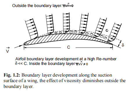
Two flow layers are distinguished: (1) a very thin layer close to the surface, called the boundary layer, where the viscosity effect is predominant and (2) an external layer where the viscosity maybe neglected. As a result, the fluid outside the boundary layer maybe considered inviscid. In this case, the Navier-Stokes equation is reduced to the Euler equation of motion that can be solved. Prandtl [3] was the first to establish a concept that couples the solution of the external inviscid layer with the solution of the viscous boundary layer by developing the boundary layer theory. Using a set of assumptions that were based on a series of comprehensive experimental studies, Prandtl [3] and von Kármán [4] significantly simplified the governing system of partial differential equations and derived an integral method to solve for boundary layer momentum deficiency thickness for incompressible steady flow. Although the integral method is capable of providing useful information about the boundary layer integral parameters such as momentum thickness or wall friction, it is not able to provide detail information about the velocity distribution within the boundary layer. Likewise, cases with flow separation cannot be treated. Furthermore, it contains several empirical correlations that have to be adjusted from case to case. To partially circumvent  the  above  deficiencies,  the  integral  method  can  be  replaced  by  a differential method.

Although the introduction of boundary layer theory was a major breakthrough in fluid mechanics, its field of applications is limited. With the introduction of powerful numerical methods and high speed computers, it is now possible to solve the Navier- Stokes equations for laminar (see Section 1.3.1) flows. To find solutions for turbulent (see Section 1.3.1) flows, the equations are averaged leading to Reynolds averaged Navier-Stokes equations (RANS). The averaging process creates a new second order tensor called the Reynolds stress tensor, with nine unknowns. The numerical solution of RANS, however, requires modeling the Reynolds stress tensor. In the last three decades,  a  variety  of turbulence models have been  developed  including  single algebraic and multi-equation models. The trend in computation fluid dynamics goes toward a direct numerical simulation (DNS) of Navier-Stokes equations, avoiding time averaging and turbulence modeling altogether.

原资料见附件

免责声明：

本页面/内容部分素材来源于互联网公 开 信 息，旨在传递更多信息，不代表本平台立场。

版权归原作者或机构所有，如涉及侵权，请通过平台联系我们，我们将在核实后第一时间处理。

本平台对转载内容的真实性、准确性不作任何保证，用户需自行判断并承担使用风险。