基于 MATLAB 的数字信号处理应用算法集-电子书-199页

基于 MATLAB 的数字信号处理应用算法集(Springer Algorithm collection for DSP Using MATLAB 2007)
摘要:
本书是 ADI 官方出品的混合信号与 DSP 设计权威技术手册,系统讲解模数 / 数模转换、采样系统、数字滤波、FFT 及 DSP 硬件实现全流程。内容涵盖 ADC/DAC 架构与动态性能分析、信噪比计算、采样与抗混叠滤波、Sigma-Delta 转换器、FIR/IIR 滤波器设计、多速率处理及自适应滤波。重点解析 AD 转换中的信噪比、失真与噪声优化方法,详解 ADI DSP 芯片架构与指令优化,配套大量工程实例与设计准则,覆盖通信、音频、传感器信号调理等应用,为混合信号系统与 DSP 工程开发提供完整实践指南。
Algorithm Collections for Digital Signal Processing Applications Using Matlab
E.S. Gopi
National Institute of Technology, Tiruchi, India
空springer
A C.I.P. Catalogue record for this book is available from the Library of Congress.
ISBN 978-1-4020-6409-8 (HB)
ISBN 978-1-4020-6410-4 (e-book)
Published by Springer,
P.O. Box 17, 3300 AA Dordrecht, The Netherlands.
www.springer.com
Printed on acid-free paper
All Rights Reserved © 2007 Springer
No part of this work may be reproduced, stored in a retrieval system, or trans mitted in any form or by any means, electronic, mechanical, photocopying, microfilming, recording or otherwise, without written permission from the Publisher, with the exception of any material supplied specifically for the purpose of being entered and executed on a computer system, for exclusive use by the purchaser of the work.
This book is dedicated to my Wife G.Viji
and my Son V.G. Vasig
Preface
The Algorithms such as SVD, Eigen decomposition, Gaussian Mixture Model, PSO, Ant Colony etc. are scattered in different fields. There is the need to collect all such algorithms for quick reference. Also there is the need to view such algorithms in application point of view. This Book attempts to satisfy the above requirement. Also the algorithms are made clear using MATLAB programs. This book will be useful for the Beginners Research scholars and Students who are doing research work on practical applications of Digital Signal Processing using MATLAB.
Acknowledgments
I am extremely happy to express my thanks to the Director Dr M.Chidambaram, National Institute of Technology Trichy India for his support. I would also like to thank Dr B.Venkatramani, Head of the Electronics and Communication Engineering Department, National Institute of Technology Trichy India and Dr K.M.M. Prabhu, Professor of the Electrical Engineering Department, Indian Institute of Technology Madras India for their valuable suggestions. Last but not least I would like to thank those who directly or indirectly involved in bringing up this book sucessfully. Special thanks to my family members father Mr E.Sankara subbu, mother Mrs E.S.Meena, Sisters R.Priyaravi, M.Sathyamathi, E.S.Abinaya and Brother E.S.Anukeerthi.
Thanks
E.S.Gopi
Chapter 1 ARTIFICIAL INTELLIGENCE
Algorithm Collections
1. PARTICLE SWARM ALGORITHM
Consider the two swarms flying in the sky, trying to reach the particular destination. Swarms based on their individual experience choose the proper path to reach the particular destination. Apart from their individual decisions, decisions about the optimal path are taken based on their neighbor’s decision and hence they are able to reach their destination faster. The mathematical model for the above mentioned behavior of the swarm is being used in the optimization technique as the Particle Swarm Optimization Algorithm (PSO).
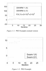
For example, let us consider the two variables ‘x’ and ‘y’ as the two swarms. They are flying in the sky to reach the particular destination (i.e.) they continuously change their values to minimize the function (x-10)2+(y- 5)2. Final value for ‘x’ and ‘y’ are 10.1165 and 5 respectively after 100 iterations.
The Figure 1-1 gives the closed look of how the values of x and y are changing along with the function value to be minimized. The minimization function value reached almost zero within 35 iterations. Figure 1-2 shows the zoomed version to show how the position of x and y are varying until they reach the steady state.
1.1 How are the Values of ‘x and y’ are Updated in Every Iteration?
The vector representation for updating the values for x and y is given in Figure 1-3. Let the position of the swarms be at ‘a’ and ‘b’ respectively as shown in the figure. Both are trying to reach the position ‘e’. Let ‘a’ decides to move towards ‘c’ and ‘b’ decides to move towards ‘d’.
The distance between the position ‘c’ and ‘e’ is greater than the distance between ‘d’ and ‘e’. so based on the neighbor’s decision position ‘d’ is treated as the common position decided by both ‘a’ and ‘b’ . (ie) the position ‘c’ is the individual decision taken by ‘a’, position ‘d’ is the individual decision taken by ‘b’ and the position ‘d’ is the common position decided by both ‘a’ and ‘b’.
1. Artificial Intelligence
‘a’ based on the above knowledge, finally decides to move towards the position ‘g’ as the linear combination of ‘oa ’ , ‘ac ’ and ‘ad’. [As ‘d ’ is the common position decided].The linear combination of ‘oa’ and scaled ‘ac’ (ie) ‘af’ is the vector ‘of’. The vector ‘of’ combined with vector ‘fg’ (ie) scaled version of ‘ad’ to get ‘og’ and hence final position decided by ‘a’ is ‘g’.
Similarly, ‘b’ decides the position ‘h’ as the final position. It is the linear combination of ‘ob’ and ‘bh’(ie) scaled version of ‘bd’. Note as ‘d’ is the common position decided by ‘a’ and ‘b’, the final position is decided by linear combinations of two vectors alone.
Thus finally the swarms ‘a’ and ‘b’ moves towards the position ‘g’ and ‘h’ respectively for reaching the final destination position ‘e’ . The swarm ‘a’ and ‘b’ randomly select scaling value for linear combination. Note that ‘oa’ and ‘ob’ are scaled with 1 (ie) actual values are used without scaling. Thus the decision of the swarm ‘a’ to reach ‘e’ is decided by its own intuition along with its neighbor’s intuition.
Now let us consider three swarms (A,B,C) are trying to reach the particular destination point ‘D’. A decides A’, B decides B’ and C decides C’ as the next position. Let the distance between the B’ and D is less compared with A’D and C’ and hence, B’ is treated as the global decision point to reach the destination faster.
Thus the final decision taken by A is to move to the point, which is the linear combination of OA, AA’ and AB’. Similarly the final decision taken by B is to move the point which is the linear combination of OB, BB’. The final decision taken by C is to move the point which is the linear combination of OC, CC’ and CB’.
1.2 PSO Algorithm to Maximize the Function F (X, Y, Z)
1. Initialize the values for initial position a, b, c, d, e
2. Initialize the next positions decided by the individual swarms as a’, b’, c’ d’ and e’
3. Global decision regarding the next position is computed as follows. Compute f (a’, b, c, d, e), f (a, b’, c, d, e), f (a, b, c’, d, e), f (a, b, c, d’, e) and f (a, b, c, d, e’). Find minimum among the computed values. If f (a’, b, c, d, e) is minimum among all, the global position decided regarding the next position is a’. Similarly If f (a, b’, c, d, e) is minimum among all, b’ is decided as the global position regarding the next position to be shifted and so on. Let the selected global position is represented ad ‘global’
4. Next value for a is computed as the linear combination of ‘a’ , (a’-a) and (global-a) (ie)
• nexta = a+ C1 * RAND * (a’ –a) + C2 * RAND * (global –a )
• nextb = b+ C1 * RAND * (b’ –b) + C2 * RAND * (global –b)
• nextc = c+ C1 * RAND * (c’ –c) + C2 * RAND * (global –c )
• nextd = d+ C1 * RAND * (d’ –d) + C2 * RAND * (global –d )
• nexte = e+ C1 * RAND * (e’ –e) + C2 * RAND * (global –e )
5. Change the current value for a, b, c, d and e as nexta, nextb, nextc, nextd and nexte
6. If f (nexta, b, c, d, e) is less than f (a’, b, c, d, e) then update the value for a’ as nexta, otherwise a’ is not changed.
If f (a, nextb, c, d, e) is less than f (a, b’, c, d, e) then update the value for b’ as nextb, otherwise b’ is not changed
If f (a, b, nextc, d, e) is less than f (a, b, c’, d, e) then update the value for c’ as nextc, otherwise c’ is not changed
If f (a, b, c, nextd, e) is less than f (a, b, c, d’, e) then update the value for d’ as nextd, otherwise d’ is not changed
If f (a, b, c, d, nexte) is less than f (a, b, c, d, e’) then update the value for e’ as nexte, otherwise e’ is not changed
7. Repeat the steps 3 to 6 for much iteration to reach the final decision.
The values for ‘c1’,’c2’ are decided based on the weightage given to individual decision and global decision respectively.
Let Δa(t) is the change in the value for updating the value for ‘a ’ in tth iteration, then nexta at (t+1)th iteration can be computed using the following formula. This is considered as the velocity for updating the position of the swarm in every iteration.
nexta (t+1) = a (t) + Δa(t+1) where
Δa(t+1) = c1 * rand * (a ’ –a ) + c2 * rand * ( global –a ) + w(t)* Δa(t)
‘w ( t )’ is the weight at tth iteration. The value for ‘w’ is adjusted at every iteration as given below, where ‘iter’ is total number of iteration used.
w(t+1)=w(t)-t*w(t)/(iter).
Decision taken in the previous iteration is also used for deciding the next position to be shifted by the swarm. But as iteration increases, the contribution of the previous decision is decreases and finally reaches zero in the final iteration.
1.3 M – program for PSO Algorithm
psogv .m
function [value]=psogv(fun,range,ITER) %psogv.m
%Particle swarm algorithm for maximizing the function fun with two variables x %and y.
%Syntax
%[value]=psogv(fun,range,ITER) %example
%fun='f1'
%create the function fun.m %function [res]=fun(x,y)
%res=sin(x)+cos(x);
%range=[-pi pi;-pi pi];
%ITER is the total number of Iteration error=[];
vel1=[];
vel2=[];
%Intialize the swarm position swarm=[];
x(1)=rand*range(1,2)+range(1,1);
y(1)=rand*range(2,2)+range(2,1);
x(2)=rand*range(1,2)+range(1,1);
y(2)=rand*range(2,2)+range(2,1);
%Intialize weight w=1;
c1=2;
c2=2;
%Initialize the velocity v1=0;%velocity for x
v2=0;%velocity for y for i=1:1:ITER
[p,q]=min([f1(fun,x(2),y(1)) f1(fun,x(1),y(2))]);
if (q==1)
capture=x(2); else
capture=y(2); end
v1=w*v1+c1*rand*(x(2)-x(1))+c2*rand*(capture-x(1));
v2=w*v2+c1*rand*(y(2)-y(1))+c2*rand*(capture-y(1)); vel1=[vel1 v1];
vel2=[vel2 v2];
%updating x(1) and y(1)
x(1)=x(1)+v1;
y(1)=y(1)+v2;
%updating x(2) and y(2)
if((f1(fun,x(2),y(1)))<=(f1(fun,x(1),y(1))))
x(2)=x(2); else
x(2)=x(1);
end;
if((f1(fun,x(1),y(2)))<=(f1(fun,x(1),y(1))))
y(2)=y(2); else
y(2)=y(1); end
error=[error f1(fun,x(2),y(2))];
w=w-w*i/ITER;
swarm=[swarm;x(2) y(2)];
subplot(3,1,3)
plot(error,'-')
title('Error(vs) Iteration');
subplot(3,1,1)
plot(swarm(:,1),'-')
title('x (vs) Iteration');
subplot(3,1,2)
plot(swarm(:,2),'-')
title('y (vs) Iteration');
pause(0.2)
end
value=[x(2);y(2)];
f1.m
function [res]=f1(fun,x,y);
s=strcat(fun,'(x,y)');
res=eval(s);
更多内容见附件
免责声明:
本页面/内容部分素材来源于互联网公 开 信 息,旨在传递更多信息,不代表本平台立场。
版权归原作者或机构所有,如涉及侵权,请通过平台联系我们,我们将在核实后第一时间处理。
本平台对转载内容的真实性、准确性不作任何保证,用户需自行判断并承担使用风险。