Coarse-grained physical modeling of complex flow

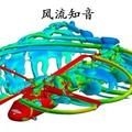
风流知音(FLOWS:Physics & beyond)【物理建模专栏(FOCUS ON PHYSICAL MODELING)】

Coarse-grained physical modeling of complex flow: from cellular automata to discrete Boltzmann

CFDPM (2018)1041

Coarse-grained physical modeling of complex flow: from cellular automata to discrete Boltzmann

--- To the Shanghai symposium on statistical physics and complex systems in memory of Prof.HAO Bailin, academician of Chinese Academy of Sciences, organized by Prof. FANG Haiping

Aiguo Xu

 1. Institute of Applied Physics and Computational Mathematics, Beijing 100088, China

2.Center for Applied Physics and Technology, Peking University, Beijing 100871,China

Abstract: It is one of the main lines of physics research to grasp the profound behavior through simple model. The development from the cellular automata to lattice Boltzmann and then to discrete Boltzmann for complex flow is briefly introduced from the perspective of physics.

Uniform fluids remain at rest or moving at the same speed along a straight line when in mechanical equilibrium.  Nearly all flowsin our daily lives and in industrial processes are in non-equilibrium. The non-equilibriumflow has various forms, and its complexity in creases sharply with the increaseof deviation from thermodynamic equilibrium. For such kind of complex flow, we can only gradually carry out research and gradually enrich understanding. It is one of the main lines in the study of fluid physics, to construct some coarse-grained model which catches the main points for specific problem and then try to understand the part of profound flow behavior through the simple model.

Cellular Automata

From the perspective of physics, cellular automata is a coarse-grained model, also known as lattice gas cellular automata (LGCA) or lattice gas model (LGM).

It is meaningful to mention that using lattice model has a long history in statistical physics and some of the most important problems in statistical physics are defined for cases where particles are confined to lie on the sites of a lattice, for example, a square, triangular, or hexagonal lattice in two dimensions or a simple cubic, face centered cubic, or body centered cubic lattice in three dimensions. Often these models either have an exclusion rule which forbids multiple occupancy of a siteor have a variable on each site which takes on a discrete number of values. An example is referred to the early work, “Statistical theory of equations of state and phase transition. II. lattice gas and Ising model” published in Physical Review in 1952 by T. D. Lee and C. N. Yang.

The basic idea of lattice gas model for fluid is as follows: a real fluid is made up of a large number of particles. However, the form of hydrodynamic differential equations does not depend on the details of microscopic processes, but only on microscopic conservation laws and symmetries (only some transport coefficients such as viscosity depend on microscopic details). Based on this assumption, people began to use the simple discrete model as an idealized model of continuous fluid system. Such a model is usually composed of a back ground grid, a group of “virtual particles” distributed on grid nodes and a set of simple rules. Where, (i) the background grid provides the coarsening coordinates of the space, (ii) each particle distributed on the grid node has the same mass and only a few motion directions and velocities bound to the grid point connection mode, (iii) the common simple rule is: in a time step, a particle can only move from the current lattice point to the adjacent lattice point along the line direction of the lattice point. This process is called “propagation”. When particles from different directions meet at a lattice point, they “collide”. The collision rule is designed to ensure the local conservations of mass, momentum and energy before and after the collision.To simulate continuous fluid system, especially in order to make symmetry, broken at the micro level, restoration on macroscopic, the lattice gas model must meet some symmetry constraints. There have been various, interesting and illuminating lattice gas models throughout history.

The physical image of lattice gas model is simple, intuitive and easy to program.It plays an important role in the rough simulation of fluid behavior, especially complex fluid behavior. The flexibility of the lattice gas model gives birth to its two future development directions: (i) numerical solver of Navier-Stokes and other kinds of Partial Differential Equations (PDEs) and (ii) coarse-grained physical modeling of non-equilibrium complex flows.

Lattice Boltzmann

Lattice Boltzmann method (LBM) is developed, through several main evolutions, on the basis of cellular automata method. The simplicity and flexibility of the discrete rule in the lattice gas model make the method attractive. However, it is understandable that they also make problems. The flow behaviors presented by the LGM show difference from those described by the continuous model represented by Euler equations and/or Navier-Stokes equations. The reliability of the continuous model in its applicable range has been tested by so many practices, so extensive attention was attracted to the reasonable construction of lattice gas model. In the following few years, after the introduction of local equilibrium distribution function, linear collision operator and single relaxation time model, the lattice gas model gradually developed into the form of the lattice Boltzmann model commonly used in the literature. Subsequently, it was found that the lattice Boltzmann equation can be regarded as an ingenious discrete form of the single relaxation time linearization Boltzmann equation in time, space and particle velocity space. Subsequently, the multiple relaxation time model has been studied extensively. As the convection term of Boltzmann equation can also be calculated in a more flexible way according to needs, the so-called finite difference lattice Boltzmann, finite volume lattice Boltzmann, finite element lattice Boltzmann and so on appear. Accordingly, the one  developed from the lattice gas model and inherited the simple physical image of “propagation collision” is often referred to as the standard lattice Boltzmann model.

Due to the simple physical image and convenience in coding, the standard LBM  attracted extensive interest in various fields. Researchers with different knowledge structures and backgrounds developed and are developing the LBM along their research directions according to their own interests. Roughly speaking, the purpose of constructing LBM or expectations for the LBM can be divided into two categories: (i) new numerical solver for PDE(s),such as the Navier-Stokes, and (ii) kinetic modeling method for non-equilibrium complex flows.

We first introduce the LBM working as PDE(s) solver. It is the one occupying the most of existing LBM literature. As for the LBM solving hydrodynamic equations, the idea of this method is greatly different from those of traditional computational fluid dynamics: In the traditional fluid simulation, the governing equations are discrete fluid equations (including mass conservation equation, momentum conservation equation and energy conservation equation). In the lattice Boltzmann simulation, the governing equation is the discrete Boltzmann equation. The results of LBM simulation agree with the fluid equations to be solved in the range of numerical error. The theoretical basis for the effectiveness of the LBM is as follows: according to Chapman-Enskog multi-scale analysis, the lattice Boltzmann equation can recover the hydrodynamic equations in the continuum limit.

From the perspective of mathematics, Chapman-Enskog multi-scale analysisis actually as below: regard the distribution function f, time derivative and spatial derivative as functions of Knudsen number Kn, then do Taylor expansion at Kn = 0, substitute them into the Boltzmann equation, then respectively for three kinetic moments, density, momentum and energy, to get the hydrodynamic equations. When Knudsen number is small, and amplitudes of third order and above are so small that can be neglected, the zero order, first order and second order energy kinetic moments of Boltzmann equation are just the mass, momentum and energy equation of Burnett equation. When Knudsen number is reduced so that the terms in the second and higher orders can be neglected, the zero order, first order and second order energy kinetic moments of Boltzmann equation are just the mass, momentum and energy equation of Navier-Stokes equations. When Knudsen number is further reduced, all the small quantities in the first order and above orders can be ignored, then the zero order, first order and second order energy kinetic moments of Boltzmann equation are just the mass, momentum and energy equation of Euler equations.

The early LBM was mainly used to solve the incompressible Navier-Stokes equations, that is, in the case of Knudsen number Kn being small, the LBM simulation can give the results consistent with the incompressible Navier-Stokes equations within the range of numerical error. Soon it was found that, as long as one can find a simulation control quantity, to correspond to the Knudsen number, then extend the concepts of distribution function and kinetic moments according to the need of solving equations (for example, the sum of all discrete “distribution function” is equal to the quantity which needs to be solved), some other kinds of PDEs can be solved by the lattice “Boltzmann equation” with appropriate modifications. Therefore, the lattice “Boltzmann” method of some other partial differential equations has also attracted wide interest. It should be pointed out that : (i)the “distribution function” and “kinetic moment” may no longer have the physical meanings of distribution function and kinetic moment in statistical physics. Accordingly, the extended “Boltzmann equation” may no longer be the Boltzmann equation in non-equilibrium statistical physics that describes thermodynamic non-equilibrium behaviors. That is, they are only some “distribution functions” in form, “kinetic moments” in form, “Boltzmann equation” in form, just a continuation of the names for convenience.(ii) compared with the coarse-grained physical model, Discrete Boltzmann Model (DBM), which will be introduced below, the algorithm design of LBM for solving PDEs may be free from the rigid rule for physical correspondence that DBM must obey, which can be regarded as the flexibility of the PDE solver study compared with the physical modeling study.

From the perspective of physical modeling of complex systems, lattice gas cellular automata model and lattice Boltzmann method themselves are some kinds of coarse-grained physical models. In addition to the continuous fluid system, it is also applicable to the rarefactive fluid system with significant mesoscopic and non-equilibrium effects. Despite this, it is a pity to see that the LBM working as mesoscopic and non-equilibrium physical modeling has not obtained so rapid development over the past decades. In the existing literature, most of, in fact nearly all,  “lattice Boltzmann methods” appear as the numerical solvers of some partial differential equations, so the “lattice Boltzmann method” has been generally accepted as a new numerical solution method of partial differential equations. At the same time, since most of the “lattice Boltzmann methods” in literature are referred to the standard LBM, LBM is often the symbol of the standard lattice Boltzmann method for solving partial differential equation(s).

For non-equilibrium flow kinetics modeling, there are also two categories. One category mainly concerns the conserved kinetic moments, the density, momentum and energy and their evolutions. In the other category, not only the three conservative moments but also some closely related non-conservative kinetic moments are taken into account. Surely, the second category can present a more complete description of the non-equilibrium state and its evolution, from which we get more meaningful physical information. In studies on the second category, investigating the non-equilibrium behavior plays a central role. For example, through the differences between non-conservative kinetic moments of f and f ^eqwhich is the corresponding equilibrium distribution function, the irreversible mechanism for entropy increase can be studied, and the influence of current non-equilibrium state on the flow behavior in next step can be studied. For the second category of kinetic modeling method of non-equilibrium flow behavior, based on the following two facts, (i) it generally no longer uses the simple physical image “propagation collision” inherited from the “lattice gas” model, and consequently, “lattice” in the method name has lost its original meaning/indication and sometimes it is misleading; (ii) it still uses the discrete Boltzmann equation,  it is gradually referred to as discrete Boltzmann modeling/model/method (DBM) in recent literature. There is no special constraint on discrete scheme for spatial derivative and time integral method of control equation in DBM. The discrete schemes can be reasonably selected according to specific situations. The “discretization” here refers only to the discretization of molecular velocity space.

Discrete Boltzmann

The following describes the kinetic modeling method, DBM, for non-equilibrium flows. The physical world is infinitely divisible. The definition of microscopic, mesoscopic and macroscopic is relative. In the description of a fluid system, the microscopic description generally refers to the one based on molecular dynamics, which means, the smaller structure and behaviors within molecules are not explicitly considered in the description of this level. The simulation tool is, of course, the well-known molecular dynamics simulation. The establishment of interaction potential between molecules is the key step for the model construction. The effective radius interception is the key step for practical numerical calculation. Macroscopic description generally refers to the description of continuous medium modeling based on Euler equations and Navier-Stokes equations. At this level, the behavior of the system concerned is characterized by physical quantities such as density, velocity, temperature, pressure, stress, and heat flow. The governing equations are the evolution equations of fluid representing the conservations of mass, momentum and energy, where the constitutive relations are often given by experience or phenomenological treatments. Since the non-equilibrium statistical physics bridges microscopic molecular and macroscopic continuous descriptions, it is often referred to as mesoscopic description. Among the basic equations of non-equilibrium statistical physics,the most used in describing flow behavior is the Boltzmann equation. In such a mesoscopic kinetic description, the starting point is the ideal gas model. The Enskog equation can be regarded as a generalization of Boltzmann equation. Suitable intermolecular forces or potentials can be introduced into the model system through the force term or the collision term.

From the perspective of physics, Knudsen number Kn is defined as the ratio of the mean free path l of molecules to the characteristic length scale L of the flow behavior we are concerned about, reflecting the relative degree of continuity or discreteness of the fluid system. According to Knudsen number Kn from small to large, the fluid is classified into continuous flow, slip flow, transition flow and free molecular flow. In principle, all the above four kinds of flow behaviors can be described by Boltzmann equation. In this sense, Boltzmann equation has cross-scale self-adaptability in physical describing non-equilibrium flows. The scale here refers to the dimensionless Knudsen number, Kn. If the characteristic scale L is taken as the scale of the system, then this Knudsen number Kn reflects the average continuous or discrete degree of the fluid system, which can be called the overall Knudsen number. Through it, one can't get information about the internal structure of the system. If we concern the internal structures of the flow system, then we need to use the local Knudsen number, that is, the characteristic scale L should be selected as the characteristic length scale of the corresponding structure, which is often defined by the density interface. For a non-equilibrium flow system, Knudsen number Kn can be defined as the ratio of the local thermodynamic relaxation time of flow system to the time scale of the flow behavior we are concerned with. Therefore, it is often used to describe the relative non-equilibrium degree of the fluid system. According to this definition, an approaching zero Knudsen number means that the flow system can nearly always be very close to its local thermodynamic equilibrium. A large Knudsen number means that the flow system can not be close to its local thermodynamic equilibrium in the flow process.

Now, we can explain the Chapman-Enskog multi-scale analysis in the language of physics as below: regard the distribution function f, spatial and temporal derivatives as functions of Knudsen number Kn; do Taylor expansion at local thermodynamic equilibrium state, then derive the evolution equations for the three kinetic moments, the density, momentum and energy. If the system is always in the local thermodynamic equilibrium state, then the macroscopic fluid equations corresponding to Boltzmann equation are Euler equations. If the system is always near the thermodynamic equilibrium state, the non-equilibrium effects of the second order and above are so weak that they can be ignored, then the macroscopic fluid equations corresponding to Boltzmann equation are Navier-Stokes equations. If the system deviates more from the thermodynamic equilibrium so that the second order non-equilibrium effects needs to be considered, but the non-equilibrium effect of the third order and above are still small enough to be negligible, then the macroscopic fluid equations corresponding to Boltzmann equation are Burnett equations. If the system further deviates from the thermodynamic equilibrium so that the higher order non-equilibrium effect needs to be considered, then the macroscopic fluid equations corresponding to Boltzmann equation are the super-Burnett equations.

From molecular dynamics to Boltzmann equation, to Burnett, Navier-Stokes and further to Euler equations, it is a process of coarser-grained modeling which is a process of physical description with gradual coarsening and gradual reduction of physical information. The stepwise transformation of the model corresponds to the system described is closer and closer to its local thermodynamic equilibrium state, and the behavior of system is more and more simple, so as to can be determined with fewer physical variables. For a certain non-equilibrium fluid system, we often need to use different models to study it. The stepwise transformation of the model corresponds to the gradual increase of the spatial-temporal scale used to observe the system, and more and more relatively smaller structures and relatively faster kinetic modes are ignored. What one gets is a flow system with the remaining larger and larger structures and slower and slower patterns. The description of complex fluid requires the cooperation of models with different levels of coarsening.

Coarse-grained physical modeling is a process which keeps only the main points and ignores the others: the physical quantities on which we study physical problems rely cannot be altered by the simplification of the model. These physical quantities which do not change due to model simplification are the invariants to be preserved in the coarse-grained physical modeling. In terms of fluid description, the invariants we need to keep are the kinetic moments of different order of distribution function. From the description of Boltzmann equation to the establishment of the present version of discrete Boltzmann model, it is necessary to undergo two steps of coarse-grained physical modeling which include the collision operator simplification and molecular velocity space discretization. Although the Boltzmann equation is already a highly coarse-grained model relative to the Liouville equation, the collision term is still too complex to be treated with in most cases, so it still has to be simplified. One way to simplify it is to introduce a formal local target distribution function, f*, and write the original collision term as a linear collision operator :（f* - f）/τ. The implication is that the effect of molecular collision is to make the distribution function f tend to f*, whose speed is controlled by the relaxation time τ. Depending on the invariants one needs to keep, f* will take a different form. Among such linear collision models, the Bhatnagar-Gross-Krook (BGK) model where f* is taken as the local equilibrium state distribution function, the Maxwellian distribution function, obtained most extensive applications due to its simplicity.

In terms of the discretization of the molecular velocity space, because the invariants that we need to preserve are some of the kinetic moments of the distribution function, all we need to do is to ensure that these kinetic moments, originally in integral form, can be equally calculated in summation form. If the speeds of different kinetic modes in the fluid system tending to their thermodynamic equilibrium differ significantly, the single relaxation time model can no longer meet the demand, and then the multi-relaxation time model needs to be constructed. In order to make each relaxation time have a clear physical meaning, the collision term calculation of the multiple relaxation time discrete Boltzmann model is generally completed first in the kinetic moment space, and then transposed back to the discrete velocity space. It should be pointed out that a direct result of model simplification is usually the reduction of application range or the decrease of detail control ability. Compared with the original Boltzmann equation, the above linear model (with single relaxation time or multiple relaxation time) is only applicable to the case where the molecular collisions are sufficient to make the distribution function f tend to the local target distribution function f*. Compared with the Boltzmann equation, the simplified process where only a few invariants are kept and grasp only the principal points according to the research need makes some uncertainty to the un-guaranteed kinetic behavior.

In practical applications, one can determine the invariants to be guaranteed according to the research requirements of specific problem, and construct the simplest discrete Boltzmann model to meet the need. Better non-equilibrium state description, non-equilibrium effect detection, extraction and analysis are the main objectives of discrete Boltzmann modeling. Thus, discrete Boltzmann modeling consists of three steps: (i) simplification of collision operator, (ii) discretization of particle velocity space, (iii) description of non-equilibrium state and extraction of non-equilibrium information. The first two steps are for coarse-grained modeling, and the third is the core of the modeling method.

Flowchart of DBM construction

The discrete Boltzmann method provides two sets of non-equilibrium behavior description tools: one is to directly compare the non-conservative kinetic moments of the distribution function and the corresponding local equilibrium state distribution function, and the other is to use the viscous stress and heat flux obtained by Chapman-Enskog multi-scale analysis. The former describes the specific non-equilibrium state, while the latter describes the influence of the current non-equilibrium state on the macro-evolutionary behavior of the system in next step. The former description is relatively detailed, while the latter description is relatively coarsening. The study of non-equilibrium behavior is helpful to understand the linear and nonlinear constitutive relations in macroscopic fluid description. In the actual research process, the relation between the non-equilibrium quantities provided by the former and the interested physical quantity (such as entropy) can be established, or the correlation, similarity and so on can be further defined between two non-equilibrium states or even two non-equilibrium flow processes. In the case of entropy, the main mechanism causing entropy increase and their relative importance can be probed. 

Physical modeling and algorithm design are two indispensable steps in numerical experimental study. The error resulted from the physical modeling cannot be compensated by the improved algorithm precision. The non-equilibrium behaviors at the macroscopic flow level are usually described by the fluid dynamics equations corresponding to mass conservation, momentum conservation and energy conservation. The physical precision of the hydrodynamic model depends largely on the rationality of the constitutive relation. The understanding of the kinetic mechanism of nonlinear constitutive relations requires investigating the thermodynamic non-equilibrium behaviors that are most closely related to macroscopic flows.

From the perspective of mathematical modeling, the typical difference between the discrete Boltzmann model and the traditional hydrodynamic model is to replace the original Navier-Stokes equations with the discrete Boltzmann equation. However, from the perspective of physical modeling, this substitution has meaningful “gain”: a discrete Boltzmann model is roughly equivalent to a continuous hydrodynamic model plus a coarse-grained model of related thermodynamic non-equilibrium behavior. The continuous hydrodynamic model can be and can also be beyond the Navier-Stokes equations. The discrete Boltzmann model has some extent of cross-scale self-adaptability in describing non-equilibrium flow processes. Via discrete Boltzmann model, the main mechanisms of entropy increase and their relative importance in the process of complex flow can be conveniently studied. New physical insights on non-equilibrium behavior brought by discrete Boltzmann model has been used in the target area for the recovery of the main characteristics of real distribution function and consequently more accurate description of the specific non-equilibrium status,  used in multiphase flow simulations for physical identifying various interfaces and corresponding tracking scheme design, used in the phase separation study for physical criteria for dividing the two stages (spinodal decomposition and domain growth), used in complex flows for discriminating shock wave in ordinary fluid from that in plasma, used in the hydrodynamic instability study for helping understand the mixing processes of material and energy, the effects of compressibility,  and so on. In addition to the more accurate description of the non-equilibrium behavior in the process of complex flows,the new insights brought by the discrete Boltzmann model can directly improve the macroscopic modeling of the corresponding physical system.

LBM numerical solver versus DBM physical modeling

LBM numerical solver for partial differential equations concerns computing efficiency and should present results being loyal to the original model. The DBM physical modeling research mainly focuses on the points where the new model surpasses the original model in terms of physical description capability according to the research demand of specific problems. Difference in research purposes leads to different principles to be followed in the construction of the methods. In the numerical experiments based on LBM solving PDE(s), what the system behavior description depends on is still the original model. In other words, the starting point of the study is the original model, LBM here is just a numerical tool to obtain numerical solutions of the original model. In the numerical experiments based on DBM, the behavior description of the system depends on the DBM model, instead of the original hydrodynamic model. In the DBM simulation, the discrete numerical schemes are selected as required, which is a compromise between the physical gain and numerical cost. DBM construction mainly includes three steps: (i) simplification of collision term, (ii) discretization of particle velocity space, (iii) non-equilibrium state description and non-equilibrium information extraction. The existence of the third step is not only a further extension to the first two steps, but also to put forward more strict physical requirements to the entire modeling process: all control equation(s) and all the kinetic moment relations used in the model construction must be consistent with the theory of non-equilibrium statistical physics, not like some LBMs for solving PDE(s) where one can construct lattice “Boltzmann equation” in form and design artificial “kinetic moment” which does not possess a clear physical correspondence.

In brief, LBM for solving PDE(s) concerns the loyalty and efficiency, while DBM concerns two other points, larger application scale than molecular dynamics and more meaningful kinetic information than traditional fluid model.

References:

1. McCoy Barry M. Advanced Statistical Mechanics. Oxford university press, Oxford,  2010.

2. Lee Z D and Yang C N.  Statistical theory of equations of state and phase transition. II. lattice gas and Ising model.  Physical Review 87, 410(1952). 

3. Chopard Bastien, Droz Michel. Cellular Automata Modeling of Physical Systems. Cambridge University Press, Cambridge, 1998.

4. Succi Sauro. The Lattice Boltzmann Equation for Fluid Dynamics and Beyond. Oxford university press, Oxford,2001.

5. Guo Zhaoli, Zheng Chuguang, Li Qing, et al. Lattice Boltzmann Method for hydrodynamics. Hubei Science & Technology Press, Wuhan 2002.

6. He Yaling, Wang Yong, Li Qing. Lattice Boltzmann Method: Theory and Applications. Science Press, Beijing, 2009.

7. Huang Haibo,Sukop M.C., LuXY.  Multiphase Lattice Boltzmann Methods: Theory and Application, Wiley, 2015.

8. Xu Aiguo, Zhang Guangcai, Zhang Yudong. Discrete Boltzmann modeling of compressible flows. in: G. Z. Kyzas, A. C. Mitropoulos (Eds.), Kinetic Theory, InTech, Rijeka, 2018, Ch. 02.doi: 10.5772/intechopen.70748. URL ：

http://dx.doi.org/10.5772/intechopen.70748   

9. Xu Aiguo, Zhang Guangcai, Zhang Yudong, Gan Yanbiao. Discrete Boltzmann Modeling of Non-Equilibrium Effects in Multiphase Flows. FLOWS: Physics and Beyond,CFDPM (2018)1001. 

10. Xu Aiguo. Non-equilibrium Flows: DBM modeling and simulation. Weixin of Frontiers of Physics. 

11. Xu Aiguo. Note on DBM for Non-Equilibrium Flows. FLOWS: Physics and Beyond，CFDPM(2018)1002. 

Note: A Chinese version with slight difference is referred to “复杂流动的粗粒化物理建模: 从元胞自动机到离散玻尔兹曼”, 《京师物理》2018年8月28日