PyTorch计算应力场

本文在一个二维网格上构造一个向量场   ，用 PyTorch 的自动微分计算其变形/应变、本构关系得到应力，再根据平衡方程反推并显示等效密度   。

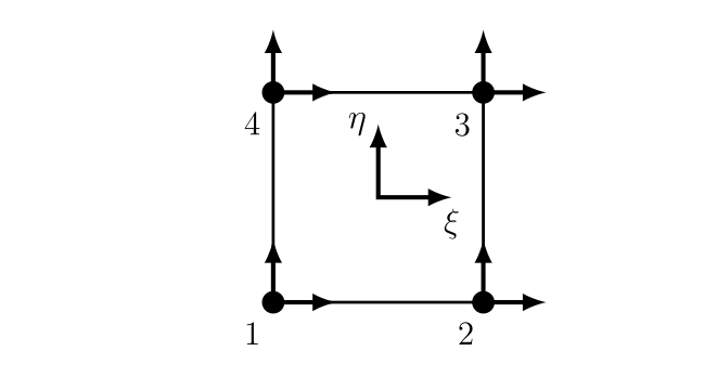
考虑一个双线性单元，如图1所示，其形函数如下：

位移场    可由位移自由度向量    建立：

计算应变    和应力   

其中    是四阶材料（本构）张量，定义为

其余分量为0。

对于 :运算 ，函数 torch.tensordot(C, strain) 将派上用场。接下来计算应力散度，以确定不平衡体力   

现在考虑如下位移场

假设材料参数   ，  ，重力加速度   （沿    负方向作用），估算材料的密度   。

1. 导入与函数定义

  import torch
import matplotlib.pyplot as plt
from torch.autograd import grad

u = lambda x, y: 0 * x ** 2 * y ** 2  
v = lambda x, y: -1.7004e-7 * y ** 2 + x ** 2 * y ** 2 * 0

• • torch：做张量和自动微分。
• • matplotlib.pyplot：画图。
• • grad：手动取梯度，等价于反向传播求偏导。

这里定义位移场分量：

实际上是0，为了让 PyTorch 知道    依赖于   ，方便后面求梯度。虽然当前结果恒为 0，但计算图里保留与输入的关系。

2. 建立网格

  nx = 5
ny = 5

x = torch.linspace(-1, 1, nx, requires_grad=True)
y = torch.linspace(-1, 1, ny, requires_grad=True)
x, y = torch.meshgrid(x, y, indexing="ij")

生成：

• •     ：从 -1 到 1，共 5 个点
• •     ：从 -1 到 1，共 5 个点
• • meshgrid(..., indexing="ij") 得到形状为 (nx, ny) 的网格，即 (5,5)

并且 requires_grad=True，表示后面可以对 x,y 求偏导。

3. 构造向量场 d = [u, v]

  d = torch.cat((u(x, y).unsqueeze(0), v(x, y).unsqueeze(0)), 0)

u(x,y) 和 v(x,y) 形状都是 (5,5)。

unsqueeze(0) 变成 (1,5,5)，再在第 0 维拼接：

  d.shape == (2, nx, ny)

即：

等价表达：

  # d[0, :, :] == u(x,y)
# d[1, :, :] == v(x,y)

4. 画向量场 quiver 图

  plt.figure(figsize=(4, 3))
plt.quiver(x.detach(), y.detach(), d[0, :, :].detach(), d[1, :, :].detach())
plt.xlabel('x')
plt.ylabel('y')
plt.title('Quiver plot of vector field (u, v)')
plt.grid(True)
plt.show()

画二维向量场箭头图。

• • .detach() 表示画图时不再需要计算图。
• • 因为     ，     只跟      有关，所以箭头主要沿 y 方向，且关于      对称。

5. 计算梯度/雅可比矩阵 dd_dx

  dd_dx = torch.zeros((2, 2, nx, ny))
dd_dx[0, 0] = grad(d[0], x, torch.ones_like(x), create_graph=True, retain_graph=True)[0] # dd_xdx
dd_dx[0, 1] = grad(d[0], y, torch.ones_like(y), create_graph=True, retain_graph=True)[0] # dd_xdy
dd_dx[1, 0] = grad(d[1], x, torch.ones_like(x), create_graph=True, retain_graph=True)[0] # dd_ydx
dd_dx[1, 1] = grad(d[1], y, torch.ones_like(y), create_graph=True, retain_graph=True)[0] # dd_ydy

这里 dd_dx 形状是：

  (2, 2, nx, ny)

它存的是向量场    对    的梯度/雅可比：

对应：

• • dd_dx[0,0] = u_x
• • dd_dx[0,1] = u_y
• • dd_dx[1,0] = v_x
• • dd_dx[1,1] = v_y

grad(output, input, grad_outputs=ones_like(...)) 计算：

但由于输出和输入同形，且 grad_outputs=ones_like(input)，实际得到逐点偏导数张量。

create_graph=True 很关键：允许对梯度再求梯度，也就是高阶自动微分。

6. 打印雅可比分量

  print(
    dd_dx[0, 0],
    dd_dx[0, 1],
    dd_dx[1, 0],
    dd_dx[1, 1]
)

打印：

7. 对称化得到小应变 eps

  eps = 0.5 * (dd_dx + dd_dx.permute((1, 0, 2, 3)))

这里把雅可比对称化：

即工程小应变张量：

由于这里   ，  ，所以：

permute((1,0,2,3)) 把前两个轴转置，即    矩阵转置，空间维度不变。

8. 材料参数和四阶弹性张量 C

  E = 210000.0
nu = 0.3

C = torch.zeros((2, 2, 2, 2)) # 4th order material tensor
C[0, 0, 0, 0] = 1.0
C[0, 0, 1, 1] = nu
C[1, 1, 0, 0] = nu
C[1, 1, 1, 1] = 1.0
C[0, 1, 0, 1] = (1.0 - nu) / 2.0
C = E / (1.0 - nu ** 2) * C

这是平面应力各向同性线弹性材料的本构张量形式。

对于平面应力：

代码中先构造无量纲部分，再乘：

其中：

• • C[0,0,0,0] 对应     
• • C[1,1,1,1] 对应     
• • C[0,0,1,1] 和 C[1,1,0,0] 对应     
• • C[0,1,0,1] 对应剪切项     

注意：这里只填了各向同性平面应力需要的几个分量，且假设无体耦合其他索引。

9. 计算应力 sig

  sig = torch.tensordot(C, eps)

更准确说是按弹性本构：

torch.tensordot(C, eps) 默认对所有匹配维度做收缩。这里 C 是 (2,2,2,2)，eps 是 (2,2,nx,ny)，实际得到 sig 形状为 (2,2,nx,ny)，表示：

即：

• • sig[0,0] =     
• • sig[1,1] =     
• • sig[0,1] =     
• • sig[1,0] =     

由于应变这里主要是   ，应力会主要由它引起。

10. 对应力再求梯度

  dsig11_dx = grad(
    sig[0, 0], x, torch.ones_like(x), create_graph=True, retain_graph=True, allow_unused=True
)[0]

dsig12_dy = grad(
    sig[0, 1], y, torch.ones_like(y), create_graph=True, retain_graph=True, allow_unused=True
)[0]

dsig21_dx = grad(
    sig[1, 0], x, torch.ones_like(x), create_graph=True, retain_graph=True, allow_unused=True
)[0]

dsig22_dy = grad(
    sig[1, 1], y, torch.ones_like(y), create_graph=True, retain_graph=True, allow_unused=True
)[0]

含义：

• • dsig11_dx = ∂σ_xx/∂x
• • dsig12_dy = ∂σ_xy/∂y
• • dsig21_dx = ∂σ_yx/∂x
• • dsig22_dy = ∂σ_yy/∂y

11. 平衡方程/残差力 f

  f = torch.zeros((2, nx, ny))
f[0] = -dsig11_dx - dsig12_dy  
f[1] = -dsig21_dx - dsig22_dy 

静力平衡如果没有加速度和体力，应满足：

分量写：

代码里：

所以可以理解为“不平衡力”或等效体力反号。若完全平衡，则 f=0。

由于这里应力来自一个给定位移场通过弹性本构算出，并不保证满足平衡，所以 f 一般不为 0。

12. 由垂直方向不平衡力估计密度

  g = 9800
rho = f[1] / g
print(rho)

假设不平衡力/体力在 y 方向来自重力：

所以：

13. 画密度等值云图

  fig, ax = plt.subplots()
cp = ax.contourf(x.detach(), y.detach(), rho.detach(), levels=12, cmap=plt.cm.jet)
fig.colorbar(cp, format="%.2e")
ax.set_aspect("equal")
fig.tight_layout()
plt.show()

完整代码

  import torch
import matplotlib.pyplot as plt
from torch.autograd import grad

u = lambda x, y: 0 * x ** 2 * y ** 2 
v = lambda x, y: -1.7004e-7 * y ** 2 + x ** 2 * y ** 2 * 0


nx = 5
ny = 5

x = torch.linspace(-1, 1, nx, requires_grad=True)
y = torch.linspace(-1, 1, ny, requires_grad=True)
x, y = torch.meshgrid(x, y, indexing="ij")


d = torch.cat((u(x, y).unsqueeze(0), v(x, y).unsqueeze(0)), 0)

plt.figure(figsize=(4, 3))
plt.quiver(x.detach(), y.detach(), d[0, :, :].detach(), d[1, :, :].detach())
plt.xlabel('x')
plt.ylabel('y')
plt.title('Quiver plot of vector field (u, v)')
plt.grid(True)
plt.show()

dd_dx = torch.zeros((2, 2, nx, ny))
dd_dx[0, 0] = grad(d[0], x, torch.ones_like(x), create_graph=True, retain_graph=True)[0]  # dd_dxdx
dd_dx[0, 1] = grad(d[0], y, torch.ones_like(y), create_graph=True, retain_graph=True)[0]  # dd_dxdy
dd_dx[1, 0] = grad(d[1], x, torch.ones_like(x), create_graph=True, retain_graph=True)[0]  # dd_dydx
dd_dx[1, 1] = grad(d[1], y, torch.ones_like(y), create_graph=True, retain_graph=True)[0]  # dd_dydy


print(dd_dx[0, 0],
      dd_dx[0, 1],
      dd_dx[1, 0],
      dd_dx[1, 1])

eps = 0.5 * (dd_dx + dd_dx.permute((1, 0, 2, 3)))


E = 210000.0
nu = 0.3

C = torch.zeros((2, 2, 2, 2))  # 4th order material tensor
C[0, 0, 0, 0] = 1.0
C[0, 0, 1, 1] = nu
C[1, 1, 0, 0] = nu
C[1, 1, 1, 1] = 1.0
C[0, 1, 0, 1] = (1.0 - nu) / 2.0
C = E / (1.0 - nu ** 2) * C


sig = torch.tensordot(C, eps)

dsig11_dx = grad(
    sig[0, 0], x, torch.ones_like(x), create_graph=True, retain_graph=True, allow_unused=True
)[0]
dsig12_dy = grad(
    sig[0, 1], y, torch.ones_like(y), create_graph=True, retain_graph=True, allow_unused=True
)[0]
dsig21_dx = grad(
    sig[1, 0], x, torch.ones_like(x), create_graph=True, retain_graph=True, allow_unused=True
)[0]
dsig22_dy = grad(
    sig[1, 1], y, torch.ones_like(y), create_graph=True, retain_graph=True, allow_unused=True
)[0]

f = torch.zeros((2, nx, ny))
f[0] = -dsig11_dx - dsig12_dy  # out of balance force in x1
f[1] = -dsig21_dx - dsig22_dy  # out of balance force in x2


g = 9810
rho = f[1] / g
print(rho)

fig, ax = plt.subplots()
cp = ax.contourf(x.detach(), y.detach(), rho.detach(), levels=12, cmap=plt.cm.jet)
fig.colorbar(cp, format="%.2e")
ax.set_aspect("equal")
fig.tight_layout()
plt.show()

总结流程

这段代码做的是：

1. 1. 定义二维向量场     ；
2. 2. 在网格上计算其梯度/变形梯度；
3. 3. 对称化得到小应变     ；
4. 4. 用平面应力各向同性弹性张量      计算应力     ；
5. 5. 计算应力散度；
6. 6. 得到不平衡力     ；
7. 7. 假设 y 方向不平衡力来自重力，反算     ；
8. 8. 可视化向量场和密度分布。