VTK库学习 | 百万级自由度有限元模型云图绘制只需0.02秒！

2月前浏览2602

温馨提示：本文字数9235，16副插图，预计阅读时间24分钟。

Python广受大家喜爱的重要原因是它有很多优秀的库，直接调用即可。针对有限元分析过程中云图的绘制，木木找了了一个非常好用的库—PyVista。PyVista是一个用于可视化工具包（VTK）的辅助模块，通过NumPy和各种方法和类提供了对VTK库的包装和直接数组访问。

项目地址：https://docs.pyvista.org/version/stable/user-guide/，该项目很容易上手，接下来教大家如何把玩这个好玩的工具！

今天的分享需要读者了解vtk的一些基础语法知识，想看历史文章：自编有限元程序如何与Paraview进行梦幻联动？，本次分享的案例数据文件都可以在知识星球内提供的《有限元基础编程百科全书》链接内下载。

官网第一个小案例

首先，先pip安装pyvista：

pip install pyvista

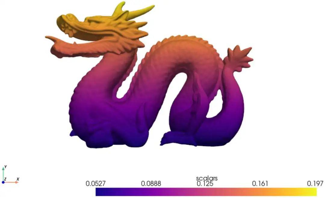
龙年先为大家画个龙年吧，官网提供的源程序只有4行，导入案例中的mesh信息，获取vtk语法中的scalars，指定绘图显示视图方向和cmap，直接出图，就是这么炫酷！

from pyvista import examples
mesh = examples.download_dragon()
mesh['scalars'] = mesh.points[:, 1]
mesh.plot(cpos='xy',cmap='plasma')

官网有非常详细的帮助文档，都是英文显示，如果大家不想去看，木木在这里整理了一些有限元云图方面常用的一些绘图设置，主要包括以下几个方面：

网格数据结构
绘图方法
云图显示
自定义绘图模板
自定义colorbar
载荷箭头、约束信息绘制
方向标志
大自由度模型测试

网格数据结构

pyvista可支持PolyData数据结构和vtk数据结构，本节先展示PolyData数据如何绘制，我主观不建议这样搞，强烈建议导入vtk文件！有关PolyData的解释可详见——https://docs.pyvista.org/version/stable/user-guide/data_model。

import pyvista as pv
import numpy as np
points = np.array([[0, 0, 0], [1, 0, 0], [0.5, 0.5, 0]])
cells = [[3, 0, 1, 2]]
mesh = pv.PolyData(points, cells)
mesh.plot(cpos='xy',show_edges=True)

以上绘制方法，我觉得颇为繁琐，不如将有限元结果写为.vtk文件，然后导入即可，之前我们是借助Paraview实现云图，现在我们直接调用pyvista进行绘制，可以达到Paraview同样的效果，且支持高度定制。使用pyvista.read(vtkfilename)进行读取，

mesh = pv.read('C3D8.vtk')
print('node number = ',mesh.n_points)
print('element number = ',mesh.n_cells)
print('node coordinate = ',mesh.points[0])
print('point_data = ',mesh.point_data)

查看有单元数：mesh.n_cells
查看节点数：mesh.n_points
节点坐标：mesh.points
单元编码：mesh.cells（缩并为一维数组）
查看SCALARS（云图变量种类）数：mesh.n_arrays
查看point data有哪些：mesh.point_data
查看point data 具体的值：mesh.point_data[’Displacement’]
查看cell data有哪些：mesh.cell_data
查看cell data 具体的值：mesh.cell_data[’AxialForce’]
也可以直接查看：mesh[’Displacement’]或mesh[’AxialForce’]
也可以自行添加cell data或者point data ：mesh.cell_data[’test’] = np.random.rand(mesh.n_cells)

绘图方法

绘图方法有两种：mesh.plot和pyvista.Plotter.add_mesh，个人喜欢后者，因为可以不断增添新特征，让我们看一下两者的效果吧，以后的教学都以后者为基础。

import pyvista as pv
from pyvista import examples
mesh = examples.load_airplane()
mesh.plot()

import pyvista as pv
from pyvista import examples
mesh = examples.load_airplane()
plotter = pv.Plotter()    
plotter.add_mesh(mesh)       
plotter.show()

云图显示

以绘制节点位移云图为例，分享pyvista的各种花式绘图技巧，在以下代码中展现了：C3D8单元的云图绘制、节点显示、单元边界显示、节点编号显示。

import pyvista as pv
mesh = pv.read('C3D8.vtk')
dargs = dict(
scalars="Displacement",
show_scalar_bar=False,
show_vertices=True,
show_edges=True,
vertex_color='red',
point_size=15,
)
pl = pv.Plotter(shape=(2, 2))  
pl.add_mesh(mesh.copy(),**dargs) 
pl.add_text("Magnitude Displacement", color='k')
pl.subplot(1, 0)
pl.add_mesh(mesh.copy(),component=0, line_width=2,**dargs) 
pl.add_text("X Displacement", color='k')
label_coords = mesh.points
pl.add_point_labels(label_coords, [f'{i+1}'for i in range(mesh.n_points)],
font_size=25, point_size=5)
pl.subplot(0, 1)
pl.add_mesh(mesh.copy(),component=1,render_points_as_spheres=True,**dargs)
pl.add_text("Y Displacement", color='k')
pl.subplot(1, 1)
pl.add_mesh(mesh.copy(),component=2,**dargs) 
pl.add_text("Z Displacement", color='k')
pl.show()

以上Python语句，相信大家只要稍微看一下就能明白，在绘图的时候可以单独设置绘图参数，比如这样：plotter.add_mesh(mesh,scalars=’Displacement’,component=0，也可以使用上述代码的形式，将绘图参数集中在drags的设置中。注意有以下几点：

component=0表示第一个分量，如果不设置的话，就表示合量Magnitude；
上图的节点显示看上去有很多没有显示，在实际绘图过程中，将图片逐渐放大后，每个节点的编号都会显示出来；
render_points_as_spheres=True表示将点的形状转换为3D圆球状，更具观赏性；
show_scalar_bar=False是为了后续定制colorbar，如果不设置为False，后面在你定制colorbar时，将会出现两个colorbar。

自定义colorbar

本小节将会分享如何自定义云图中的colorbar以及cmap，让云图的样式更漂亮一点。

import pyvista as pv
import numpy as np
from matplotlib.colors import LinearSegmentedColormap
colors = [
[0, 0, 255], [0, 93, 255], [0, 185, 255], [0, 255, 232],
[0, 255, 139], [0, 255, 46], [46, 255, 0], [139, 255, 0],
[232, 255, 0], [255, 185, 0], [255, 93, 0], [255, 0, 0]
]
colors = np.array(colors)/255.0
custom_cmap = LinearSegmentedColormap.from_list('custom_cmap', colors, N=12)
mesh = pv.read('C3D8.vtk')
dargs = dict(
scalars="Displacement",
show_scalar_bar=False,
show_vertices=True,
show_edges=True,
edge_color='#000080',
vertex_color='red',
point_size=15,
cmap = custom_cmap,
render_points_as_spheres=True
)
pl = pv.Plotter()  
pl.add_mesh(mesh.copy(),**dargs) 
pl.add_scalar_bar(title="U",n_labels=13,n_colors=12,fmt='%.3e',vertical=True,
width=0.05,position_x=0.03, position_y=0.5,font_family='times')
pl.show()

值得注意的是：

n_labels=13和n_colors=12表示colorbar上面分几段显示字，分几段显示颜色
custom_cmap是自定义的色谱，在这里我设置了12种颜色，色谱和Abaqus默认色谱保持一致，读者也可以设置其他python内置的cmap，如：jet
width=0.05表示colorbar的宽度，数值代表画幅的相对比例
position_y=0.5表示colorbar底面距离画幅底面的比例

自定义绘图模板

在设置绘图参数时，可以通过设置drags，也可以自定义绘图模板，下面给出的代码注释已写的非常清楚。

# -*- coding: UTF-8 -*-
import pyvista as pv
import numpy as np
from pyvista import themes
from matplotlib.colors import LinearSegmentedColormap
# 自定义色谱
colors = [
[0, 0, 255], [0, 93, 255], [0, 185, 255], [0, 255, 232],
[0, 255, 139], [0, 255, 46], [46, 255, 0], [139, 255, 0],
[232, 255, 0], [255, 185, 0], [255, 93, 0], [255, 0, 0]
]
colors = np.array(colors)/255.0
# N表示色谱离散程度
custom_cmap = LinearSegmentedColormap.from_list('custom_cmap', colors, N=12)
my_theme = pv.plotting.themes.DocumentTheme() # 开始自定义绘图模板
my_theme.cmap = custom_cmap # 使用自定义的custom_cmap
my_theme.show_edges = True# 单元边界显示
my_theme.show_vertices=True# 节点显示
my_theme.render_points_as_spheres=True# 节点显示转换为3D圆球
my_theme.edge_color='#000080'# 单元边界的颜色
my_theme.line_width=1# 单元边界宽度
my_theme.background = 'white'# 背景颜色
my_theme.colorbar_vertical.width = 0.05# colorbar宽度
my_theme.colorbar_vertical.position_x=0.03# colorbar 位置
my_theme.colorbar_vertical.position_y=0.5# colorbar 位置
my_theme.opacity=1# 透明度 0~1
my_theme.nan_color = 'darkgray'# 无穷大值的颜色显示
my_theme.window_size = [700, 500] # 画幅尺寸
my_theme.font.family = 'times'# 字体族
my_theme.title = 'FEA Result'# 画幅名字
pv.global_theme.load_theme(my_theme) # 加载自定义模板
mesh = pv.read('C3D8.vtk')
dargs = dict(
scalars="Displacement",
show_scalar_bar=False,
vertex_color='red',
point_size=15,
)
pl = pv.Plotter()  
pl.add_mesh(mesh.copy(),**dargs) 
pl.add_scalar_bar(title="U",n_labels=13,n_colors=12,fmt='%.3e',vertical = True)
pl.show()

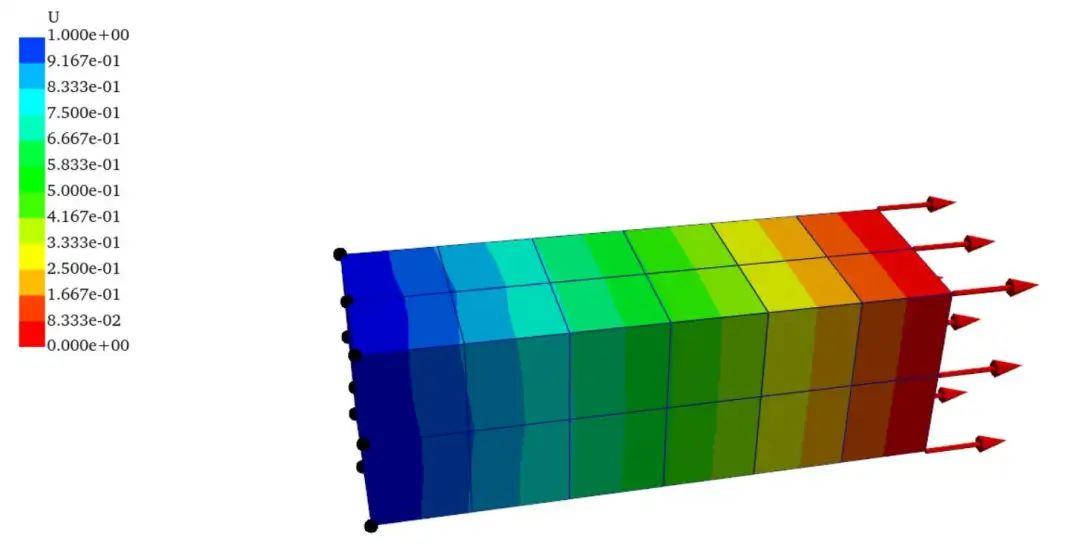
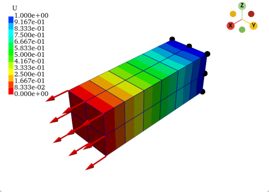
载荷箭头、约束信息绘制

为了显示边界条件的施加，我们可以添加箭头显示，值得注意的是，如果在主题模板中将show_edges设置为True，则全部的模型都讲显示边界，在这里为了美观，将箭头的边界线隐藏，在主题模板中将show_edges设置为False，模型的边界线在drags中设置。

# -*- coding: UTF-8 -*-
import pyvista as pv
import numpy as np
from pyvista import themes
from matplotlib.colors import LinearSegmentedColormap
# 自定义色谱
colors = [
[0, 0, 255], [0, 93, 255], [0, 185, 255], [0, 255, 232],
[0, 255, 139], [0, 255, 46], [46, 255, 0], [139, 255, 0],
[232, 255, 0], [255, 185, 0], [255, 93, 0], [255, 0, 0]
]
colors = np.array(colors)/255.0
# N表示色谱离散程度
custom_cmap = LinearSegmentedColormap.from_list('custom_cmap', colors, N=12)
my_theme = pv.plotting.themes.DocumentTheme() # 开始自定义绘图模板
my_theme.cmap = custom_cmap # 使用自定义的custom_cmap
my_theme.show_edges = False# 单元边界显示
my_theme.show_vertices=False# 节点显示
my_theme.render_points_as_spheres=True# 节点显示转换为3D圆球
my_theme.edge_color='#000080'# 单元边界的颜色
my_theme.line_width=1# 单元边界宽度
my_theme.background = 'white'# 背景颜色
my_theme.colorbar_vertical.width = 0.05# colorbar宽度
my_theme.colorbar_vertical.position_x=0.03# colorbar 位置
my_theme.colorbar_vertical.position_y=0.5# colorbar 位置
my_theme.opacity=1# 透明度 0~1
my_theme.nan_color = 'darkgray'# 无穷大值的颜色显示
my_theme.window_size = [700, 500] # 画幅尺寸
my_theme.font.family = 'times'# 字体族
my_theme.title = 'FEA Result'# 画幅名字
pv.global_theme.load_theme(my_theme) # 加载自定义模板
mesh = pv.read('C3D8.vtk')
dargs = dict(
scalars="Displacement",
show_scalar_bar=False,
show_edges = True,
vertex_color='red',
point_size=15,
)
pl = pv.Plotter()  
pl.add_mesh(mesh.copy(),**dargs) 
Force_node = mesh.points[range(0,9)]
Fix_node = mesh.points[range(54,63)]
direction = np.tile(np.array([1, 0, 0]), (len(Force_node), 1))
pl.add_arrows(Force_node, direction, mag=10, color='red')
pl.add_points(Fix_node, color='black',point_size=15)
pl.add_scalar_bar(title="U",n_labels=13,n_colors=12,fmt='%.3e',vertical = True)
pl.show()

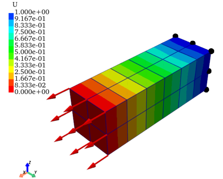
方向标志

方向标志方法有两种，代码如下，具体的参数设置我已经替大家设置完毕，看大家喜好，任选其一。

# 方向标志1
pl.add_axes(line_width=5,
cone_radius=0.6,
shaft_length=0.7,
tip_length=0.3,
ambient=0.5,
label_size=(0.4, 0.16))
# 方向标志2
pl.add_camera_orientation_widget()

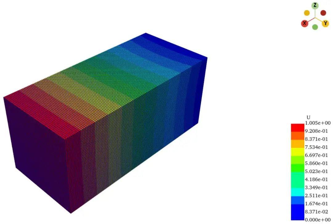
大自由度模型测试

为了测试自由度较大模型的后处理显示流畅度，我以296514个节点，282500个C3D8单元模型为例。程序读取vtk文件时间为3.52秒，云图绘制时间0.02秒，是不是相当快！

# -*- coding: UTF-8 -*-
from pyvista import examples
import numpy as np
import pyvista as pv
from pyvista import themes
import time
from matplotlib.colors import LinearSegmentedColormap
# Customized drawing templates
colors = [
[0, 0, 255], [0, 93, 255], [0, 185, 255], [0, 255, 232],
[0, 255, 139], [0, 255, 46], [46, 255, 0], [139, 255, 0],
[232, 255, 0], [255, 185, 0], [255, 93, 0], [255, 0, 0]
]
colors = np.array(colors)/255.0
custom_cmap = LinearSegmentedColormap.from_list('custom_cmap', colors, N=12)
my_theme = pv.plotting.themes.DocumentTheme()
my_theme.cmap = custom_cmap
# my_theme.cmap = 'jet'
my_theme.show_edges = True
my_theme.edge_color='#000080'
my_theme.line_width=1
my_theme.render_points_as_spheres=True
my_theme.background = 'white'
my_theme.opacity=1
my_theme.nan_color = 'darkgray'
my_theme.window_size = [600, 400]
my_theme.font.family = 'times'
my_theme.title = 'FEA Result'
my_theme.show_scalar_bar=False
pv.global_theme.load_theme(my_theme)
# Testing the time to read a .vtk file
data_start_time = time.time()
mesh = pv.read('output_C3D8.vtk')
data_end_time = time.time()
dargs = dict(
scalars="Displacements",
)
pl = pv.Plotter()
# Testing the time to plot
plot_start_time = time.time()
pl.add_mesh(mesh.copy(),  **dargs)
pl.add_scalar_bar(title="U",n_labels=13,n_colors=12,fmt='%.3e',vertical=True)
pl.add_camera_orientation_widget()
plot_end_time = time.time()
pl.show()
print("read .vtk file time: ", data_end_time - data_start_time, "s")
print("plot time: ", plot_end_time - plot_start_time, "s")