pybamm电池模型说明、案例


#
# Simulate user-defined current profile
#
import pybamm
import numpy as np
def car_current(t):
"""
Piecewise constant current as a function of time in seconds. This is adapted
from the file getCarCurrent.m, which is part of the LIONSIMBA toolbox [1]_.
References
----------
.. [1] M Torchio, L Magni, R Bushan Gopaluni, RD Braatz, and D. Raimondoa.
LIONSIMBA: A Matlab framework based on a finite volume model suitable
for Li-ion battery design, simulation, and control. Journal of The
Electrochemical Society, 163(7):1192-1205, 2016.
"""
current = (
1 * (t >= 0) * (t <= 50)
- 0.5 * (t > 50) * (t <= 60)
+ 0.5 * (t > 60) * (t <= 210)
+ 1 * (t > 210) * (t <= 410)
+ 2 * (t > 410) * (t <= 415)
+ 1.25 * (t > 415) * (t <= 615)
- 0.5 * (t > 615)
)
return current
# load model
pybamm.set_logging_level("INFO")
model = pybamm.lithium_ion.DFN()
# create geometry
geometry = model.default_geometry
# load parameter values and process model and geometry
param = model.default_parameter_values
param["Current function [A]"] = car_current
param.process_model(model)
param.process_geometry(geometry)
# set mesh
mesh = pybamm.Mesh(geometry, model.default_submesh_types, model.default_var_pts)
# discretise model
disc = pybamm.Discretisation(mesh, model.default_spatial_methods)
disc.process_model(model)
# simulate car current for 30 minutes
t_eval = np.linspace(0, 1800, 600)
solution = pybamm.CasadiSolver(mode="fast").solve(model, t_eval)
# plot
plot = pybamm.QuickPlot(solution)
plot.dynamic_plot()


.jpg?imageView2/2/h/336)