【妙趣力学|陆面体】地震导致印度洋海啸的波浪高度仿真
风流知音【妙趣力学|陆面体科技】地震导致印度洋海啸的波浪高度仿真 CFDST(2019)1016
地震导致印度洋海啸的波浪高度仿真
陆面体科技


♥ 你我永远都不会放弃爱与希望

2019.06.17
6月17日晚上22时55分在四川宜宾市长宁县发生6.0级地震!(中国地震台网正式测定)。
随后,不少市民拍摄的地震预警视频在网上广为流传。社区“大喇叭”读秒、电视自动弹出倒计时……这一地震预警系统让不少民众感到新奇,而其预警的准确性更是迅速成为网络热点。
其中,大陆地震预警网为距震中51千米的宜宾市,预警时间10秒,预估烈度5.2度。
距震中80千米的泸州市,预警时间18秒,预估烈度4.6度距震中111千米的自贡市,预警时间27秒,预估烈度4.1度;距震中124千米的毕节,预警时间31秒,预估烈度4.0度。


地震预警的重要性无可厚非,陆陆拍不出灾难片预警,但是可以讲一个仿真案例呀!在中美贸易战僵持的技术背景下,今天就不用美国的软件来讲这个案例了,我们来试试法国的开源软件Gerris Flow Solver (以下简称Gerris)。

Gerris由Stéphane Popinet创建,并由Institut Jean le Rond d'Alembert(该研究院属于巴黎索邦大学)提供支持。现在Gerris的原始开发人员现在已经将开发转移到了Basilisk,它可以完成Gerris可以做的大部分工作,甚至更多。

软件主要特点如下:
- 求解时间依赖的不可压缩变密度Euler,Stokes或Navier-Stokes方程
- 求解线性和非线性浅水波方程
- 基于流场特征的网格自适应加密
- 复杂模型的网格自动化生成
- 空间和时间二阶精度
- 不限数量的对流、扩散粒子追踪
- 可灵活加入源项
- MPI并行支持,动态负载平衡,并行可视化
- 基于VOF方法的多相流界面捕捉
- 准确的表面张力模型
- 多相电-磁流体动力学

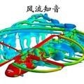
2004年印度洋海啸是由于印度-澳大利亚和印度尼西亚的安达曼板块边界发生大规模断层破裂(> 1000公里)造成的。该案例运用格里利等人的断层模型作为圣维南原理分析海啸的初始条件。图1a中的动画展示了波高的演变。追踪波前中采用了自适应方法(图1.b),地形的动态重建依据ETOPO1数据集。


(图1b)自适应动画图,图中波前峰值为海拔0.8海里和-101海里。
图2展示了断层破裂后在超过10小时的时间达到的最**浪高度。

图2:超过10小时后最**浪高度云图(以1m为显示间隔):
(a)孟加拉弯,最小值(蓝色)0m,最大值(红色)5m。
(b) 苏门答腊北部和泰国附近的细节,最小值(蓝色)0m,最大值(红色)大于8m。
最后,图3给出了在印度洋特定位置的不同时间观测波高(使用潮汐测量仪)和模拟波高的对比图。

图3:在不同潮汐表位置观测到的波高和模拟波高的对比。
备注:水平轴是断层破裂后的时间(以小时为单位)。

图4:观测波高(Jason-1卫星测高仪)和模拟波高对比。
# Segment 1
Init {} { D = 0
}
InitOkada D
{ x = 94.57
y = 3.83
depth = 11.4857e3
strike = 323
dip = 12
rake = 90
length = 220e3
    width = 130e3
    U = 18
    }
    # Initial water level is at z = D
Init
{ start = 0
}
{ P = MAX (0., D - Zb)
}
# Segment 2
    EventList
{ start = 212
step = 6
end = 272
}
{ Init {} { D = 0
}
InitOkada D
{ x = 93.90
y = 5.22
    depth = 11.4857e3
    strike = 348
dip = 12
rake = 90
length = 150e3
width = 130e3
U = 23
}
}
    # make sure the deformation is well resolved
    AdaptGradient
{ start = 212
istep = 1
end = 272
}
{ cmax = 0.05
        cfactor = 2
        minlevel = 5
maxlevel = LEVEL
    } D
    # add it to the current elevation field (only if wet)
    Init
{ start = 272
}
{ P = (P < DRY ? P : MAX (0., P D))
}
# Segment 3
    EventList
{ start = 528
step = 6
end = 588
}
    {
Init {}
{ D = 0
}
InitOkada D
{ x = 93.21
    y = 7.41
    depth = 12.525e3
    strike = 338
dip = 12
rake = 90
length = 390e3
    width = 120e3
    U = 12
        }
    }
    # make sure the deformation is well resolved
    AdaptGradient
{ start = 528
istep = 1
end = 588
}
{ cmax = 0.05
        cfactor = 2
        minlevel = 5
        maxlevel = LEVEL
    } D
    # add it to the current elevation field (only if wet)
    Init
{ start = 588
}
{ P = (P < DRY ? P : MAX (0., P D))
}
# Segment 4
    EventList
{ start = 853
step = 6
end = 913
}
{ Init {} { D = 0
}
InitOkada D
{ x = 92.60
y = 9.70
depth = 15.12419e3
strike = 356
dip = 12
    rake = 90
    length = 150e3
width = 95e3
    U = 12
     }
    }
    # make sure the deformation is well resolved
    AdaptGradient
{ start = 853
istep = 1
end = 913
}
    {
        cmax = 0.05
cfactor = 2 minlevel = 5
        maxlevel = LEVEL
    } D
    # add it to the current elevation field (only if wet)
    Init
{ start = 913
}
{ P = (P < DRY ? P : MAX (0., P D))
}
    # Segment 5
    EventList
{ start = 1213
step = 6
end = 1273
}
{ Init {} { D = 0
}
InitOkada D
{ x = 92.87
    y = 11.70
    depth = 15.12419e3
    strike = 10
dip = 12
    rake = 90
    length = 350e3
    width = 95e3
    U = 12
}
    }
[1] Hyunuk An and Soonyoung Yu. Well-balanced shallow water flow simulation on quadtree cut cell grids. Advances in Water Resources, 39:60–70, 2012.
[2] H. Glauert. The Elements of Aerofoil and Airscrew Theory. Cambridge University Press, 1926.
[3] S.T. Grilli, M. Ioualalen, J. Asavanant, F. Shi, J.T. Kirby, and P. Watts. Source constraints and model simulation of the December 26, 2004, Indian Ocean Tsunami. Journal of Waterway, Port, Coastal, and Ocean Engineering, 133:414–428, 2007.
[4] N.R. Hanson. A picture theory of theory meaning. The nature and function of scientific theories, pages 233–274, 1970.
[5] E. N. Jacobs, K. E. Ward, and R. M. Pinkerton. The characteristics of 78 related airfoil sections from tests in the variable-density wind tunnel. Technical report, NACA Technical Report 460, 1933.
[6] P.-Y. Lagrée, L. Staron, and S. Popinet. The granular column collapse as a continuum: validity of a Navier–Stokes model with a µ(i)-rheology. Journal of Fluid Mechanics, 2011.
[7] R.J. LeVeque and D.L. George. High-resolution finite volume methods for the shallow water equations with bathymetry and dry states. Advanced numerical models for simulating tsunami waves and runup, 10:43–73, 2006.
[8] L.M. Milne-Thomson. Theoretical aerodynamics (4th ed.). Dover, New York, 1973.
[9] S. Popinet. Quadtree-adaptive tsunami modelling. Ocean Dynamics, 61(9):1261–1285, 2011.
[10] C. Rosales and C. Meneveau. Linear forcing in numerical simulations of isotropic turbulence: Physical space implementations and convergence properties. Physics of Fluids, 17:095106, 2005.
[11] L. Staron and E. J. Hinch. Study of the collapse of granular columns using two-dimensional discrete-grain simulation. Journal of Fluid Mechanics, 545:1–27, 2005.
[12] J. J. Videler. Avian Flight. Oxford Ornithological Studies. Oxford University Press, 2006.
THE END
最后的最后,愿逝者安息,感恩幸存。