过冷水：分子动力学数据的Matlab处理程序设计

3年前浏览2374

过冷水诚挚邀请你加入Matlab仿真秀官方交流群进行Matlab学习、问题咨询、 Matlab相关资料下载，**：927550334

导读：MATLAB是美国MathWorks公司出品的商业数学软件，用于数据分析、无线通信、深度学习、图像处理与计算机视觉、信号处理、量化金融与风险管理、机器人，控制系统等领域。即日起，仿真秀平台将推出Matlab仿真知识圈专题，诚邀Matlab专业领域的优质内容创作者加入仿真秀创作，并优先推荐优质内容创作者加入仿真秀平台“千人万元”计划。

目前算法工匠卫通（副总工）、过冷水（电化学）博士、好学懿（电子电力）博士和伟SSS(联合物理仿真)博士都已经在仿真秀平台创作，并组建了Matlab工程师交流群(927550334)，欢迎加入。

一、写在前面

化工和材料作为社会发展的洼地一直各个方向的发展都有大量的研究者去从事，材料行业今年来呈现着高速发展的势头，在本世纪内，金属材料仍将是人类社会最主要的和不可替代的结构材料，也是产量最大、覆盖面最广的功能材料”。液态金属和液态合金最常见材料形式。材料研究者都想弄明白液态金属固溶体的结构和性质的关系。以便更好的设计出满足社会发展需求的材料。

1998年诺贝尔化学奖授予科恩和波普尔时,授奖公告附件中喊出“材料学和化学不再是纯粹的实验科学”的道理。计算实验是发展的必然产物,1953 年著名的Fermi- Pasta- Ulam的计算机实验，研究了动力学体系非线性项的微扰是如何改变单- -的周期振动行为的。1967年Orban等用分子动力学模拟一个由100 个硬球组成的体系Loschmidt做出了有说服力的解释,指出了运动方程的微观可逆性与Boltzmann的H定理所指出的宏观不可逆性是不矛盾的。

动力学模拟是研究液态结构的重要方式。民科界一直流行着这么一个传说“遇事不决量子力学”。量子力学和动力学结合就诞生了从头算分子动力学。从头算分子动力学(AIMD)计算能够获得研究体系的相关结构信息，比如：分布函数、结构因子、扩散系数、融化曲线。有物理背景的研究者应该有一个基本的认真常识，动力学模拟能够做到的是研究粒子的运动轨迹，动力学不能一步到位解决你那些奇奇怪怪的需求。你只能得到如下的一个数据文件：

11.108800 0.000000 0.000000

0.000000 11.108800 0.000000

0.000000 0.000000 11.108800

Direct configuration= 10

0.42092779 0.58594194 0.50578951

0.18475748 0.41819491 0.59613338

0.14835574 0.71785868 0.53178155

0.34971385 0.06215204 0.04694029

0.62799078 0.30549410 0.13187164

0.26709301 0.27861690 0.85821437

0.92164482 0.47341180 0.48192948

0.77994231 0.25485861 0.69514114

0.43121484 0.76988995 0.03982504

0.92373785 0.33029180 0.24657878

0.81768350 0.60132972 0.22961309

0.39420156 0.95479835 0.72730423

0.99160122 0.62915551 0.00392334

0.67489843 0.83030010 0.26653164

0.19053154 0.35526702 0.32536195

0.83555578 0.81716084 0.76528526

0.10463052 0.12816219 0.21060862

0.54511478 0.17262293 0.62753435

0.05625219 0.13802982 0.90850533

0.12998535 0.83914476 0.14942978

0.08920516 0.95744327 0.68377988

0.10764582 0.34682387 0.05297563

0.71688013 0.73362921 0.94796302

0.78657787 0.43774434 0.98078328

0.67702789 0.00551041 0.85303403

0.33513438 0.79663246 0.29237108

0.30453292 0.18409094 0.56486519

0.25671415 0.54531493 0.81768745

0.43549720 0.37284180 0.70017254

0.59961202 0.25504671 0.88326433

0.51432188 0.58065115 0.24124591

0.70332092 0.50102201 0.73685920

0.03010111 0.16861626 0.52130278

0.44122179 0.34386819 0.38741339

0.88205432 0.05299728 0.26684659

0.51824197 0.74826616 0.77912779

0.49967222 0.51884373 0.95093198

0.93215976 0.89805946 0.00837745

0.59284908 0.04688607 0.16932086

0.95386910 0.82992146 0.34561180

0.71149967 0.99905897 0.50205998

0.16565930 0.96892858 0.41765343

0.04791809 0.59552075 0.29238147

0.00532116 0.39640610 0.83319600

0.35970158 0.32677838 0.11773935

0.84071159 0.15889424 0.03466378

0.70951008 0.22317174 0.41899275

0.24450407 0.57998735 0.11248706

0.73199230 0.69513269 0.52486394

0.36583443 0.07190711 0.30529076

0.65219081 0.45075755 0.43380882

0.21476376 0.80187502 0.88158117

Direct configuration= 20

0.38416894 0.59334951 0.48113223

0.20605784 0.40652086 0.58252806

0.16541075 0.72507237 0.54536840

0.34480736 0.07889455 0.01905659

0.61625351 0.32952484 0.18925970

0.24938644 0.32687667 0.86834016

0.95046661 0.49681446 0.50286234

0.79847190 0.28187105 0.70437471

0.45750368 0.76930040 0.01299234

0.90728138 0.30200257 0.25733124

0.79923413 0.57898749 0.21324838

0.37300899 0.95694659 0.71792519

0.98131904 0.63418571 0.02162418

0.67965479 0.79341089 0.27658631

0.15910123 0.35888425 0.32975381

0.84909526 0.81828349 0.71333146

0.13576850 0.13026681 0.14249912

0.56624639 0.14282894 0.61698813

0.04734539 0.12878723 0.83091641

0.15333872 0.83937966 0.13531440

0.07271816 0.92430752 0.67754337

0.07134489 0.38783714 0.06844660

0.71693129 0.72361969 0.00366940

0.81783582 0.42276864 0.00169130

0.68736112 0.00229177 0.86676486

0.34560460 0.79050381 0.32138732

0.23581565 0.13380943 0.61545188

0.24597947 0.57692345 0.83295740

0.46447946 0.42971483 0.66563626

0.56198822 0.24389428 0.91550816

0.50038979 0.61022544 0.23094741

0.67379645 0.50917675 0.76414095

0.98944655 0.18763257 0.50592290

0.42917135 0.33124582 0.40804122

0.88919442 0.02458700 0.26925254

0.56204225 0.70683417 0.75357957

0.50369968 0.50248619 0.95976762

0.91252800 0.91230896 0.00780296

0.59170812 0.03886167 0.17693190

0.93191352 0.78340644 0.38311450

0.73863929 0.93019949 0.49991459

0.13832250 0.96087435 0.40443826

0.13894876 0.61884807 0.31237148

0.00551185 0.41883362 0.78247815

0.35957569 0.32085250 0.12169607

0.81670193 0.18147628 0.04303013

0.74416549 0.20519203 0.38614504

0.25421216 0.58105984 0.08375452

0.75402852 0.67609298 0.51937531

0.34846272 0.11933871 0.32615554

0.66609342 0.46918002 0.44827808

0.22954785 0.83873836 0.88932707

过冷水本期要给大家讲的就是怎么应用上述数据实现液态体系的结构性质的研究。

二、对分布函数g(r)&结构因子概述

1916年Debye、Scherrer首次使用x-ray衍射研究液态结构。1927年Zernike、 Prins 利用傅里叶变换理论得到了液体的径向分布函数(对分布函数)。结构因子和对分布函数相互傅里叶关系转化。

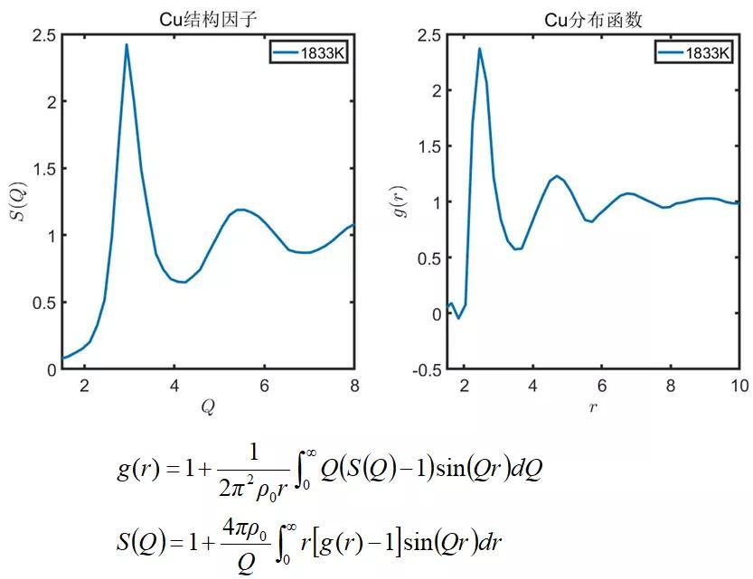
根据实验研究方法的进展是采用x射线衍射、中子衍射、电子衍射得到衍射强度曲线。然后对衍射强度曲线进行处理得到静态结构因子。

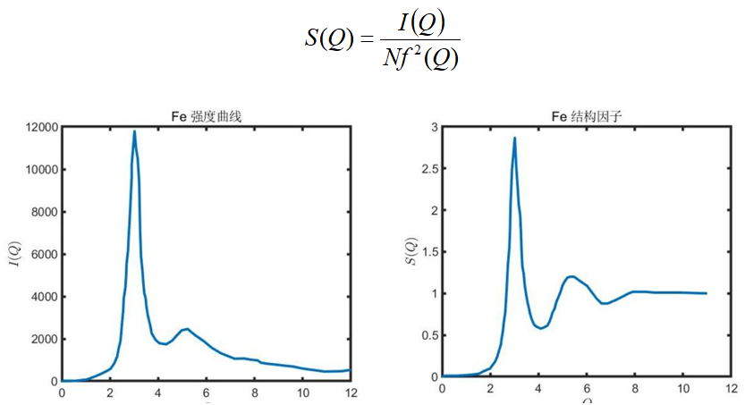
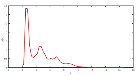
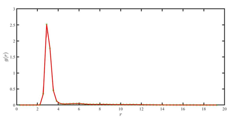
动力学模拟的流程和其是反着来的，得到原子演化轨迹坐标。根据坐标数据利用g(r)的定义：任一原子处于距离参考原子r处的几率可以得到统计形式的对分布函数公式

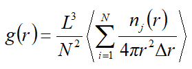
根据该函数公式我们就可以用原子坐标通过对函数进行编程化得到分布函数图像g(r)。

clear

tic

height= 9.6236000061000002;width= 9.6236000061000002;long= 9.6236000061000002;

N=54;

n=60; %划分区间个数

load('data.mat');

rc = sqrt(width^2 height^2 long^2); %搜索圆的最大半径

dr = rc/n;%确定半径区间

num = round(rc/dr);

[m1,~]=size(a);

for i=1:length(a)/N

b= a(1 (N*(i-1)):N*i,:);

Centers{i,1}=b;

end

gr=zeros(num,1);

for k=1:length(Centers)

centers=Centers{k,1};

particle_num=length(centers);

[row,col] = size(centers);

for i=1:(row-1)

centersj=centers;

centersj(i,:)=[];

Distance =sqrt((centers(i,1)-centersj(:,1)).^2 (centers(i,2)-centersj(:,2)).^2 (centers(i,3)-centersj(:,3)).^2);

for j=1:length( Distance);

distance=Distance(j,1);

if distance <= rc%计算

lane = round(distance/dr);

gr(lane) = gr(lane) 1;%做个数累计

end

%绘制径向分布函数

[row,col] = size(gr);

percent = zeros(row,1);

gobal_rho = particle_num /((3/4)*rc^3);

for i=1:row

temp = gr(i);%不同半径下的单位原内的原子个数

temp = temp / (particle_num*2*length(Centers));

temp = temp / ((4/3)*pi*((i*dr)^3-((i-1)*dr)^3));%某一个半径梯度下的局部密度

percent(i) = temp / gobal_rho;

end

%index = (1:row)/3.4;%该语句不明白什么意思

index=nonzeros(linspace(0,rc,num 1))';

percent = reshape(percent,1,row);

figure;

% plot(index,percent,'r');

xlim([0, 20]);

ylim([0, 20]);

values = spcrv([[index(1) index index(end)];[percent(1) percent percent(end)]],3)';

r=values(:,1);g=values(:,2);

figure1 = figure;

axes1 = axes('Parent',figure1);

hold(axes1,'on');

plot(r,g,'Color',[1 0 0]);

plot(index,percent,'LineWidth',3,'Color',[1 0 0]);

ylabel('$g(r)$','HorizontalAlignment','right','FontSize',20,'Interpreter','latex');

xlabel('$r$','FontSize',20,'Interpreter','latex');

box(axes1,'on');

hold(axes1,'off');

set(axes1,'FontName','Times New Roman','FontSize',16,'LineWidth',3);

toc

以上代码就只是为了实现一个公式的具体表现，可见解析公式的编程化是有多难。做动力的应该也有了解有一款软件VMD的软件也可以实现对分布函数g(r)的绘制。

过冷水在实际中发现商业软件(VMD)、material studio都可以绘制分布函数，问题在于针对相同数据源用不同软件绘制得到不完全一致的图像，究竟那个是真的？

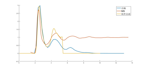
上图分别是商业软件material studio、vasp、matlab给出的分布函数图像。可以很明显的看出来基本走势是一样的，问题在于峰值走势后图像差别很大，最正确的是我自编的，其它都是采用了美化手段，在使用商业软件的时候就需要注意这问题，基本都是大体不会出错，细节上为了容易解释，让图像看上去好看一点就采用了各种近似。在此提醒仿真研究的从业人员，小心你使用的软件误导你。

三、学习相对角距离方法

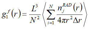
现在根据最新提出来一种叫做相对角判断的方法（RAD）可以用于确定第一配位球层，了解非晶体结构的朋友自然之道第一配位球层的意义，同样以下公式来实现的。

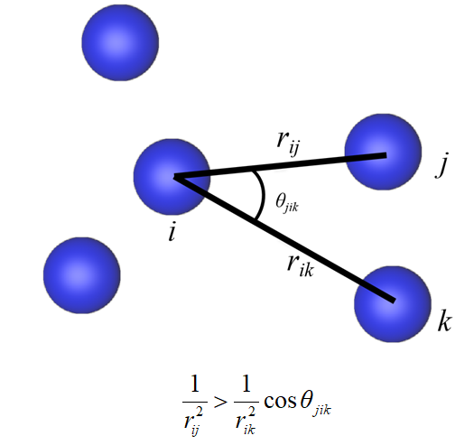
该方法给出了判断以i原子为中心,j原子在其配位层内的条件。对于原子i，如果对所有原子k满足关系式，则认为原子j是在i的配位层内，将关系式带入分布函数公式中就得到由RAD方法确定的分布函数公式

最终得到

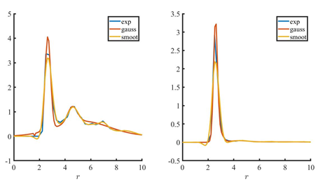
在用程序计算分布函数的时候还发现存在这么一个问题。在直接求分布函数g(r)和g(r)RAD时得到的函数图像为了求配位数是需要做积分的。以及为了让图像好看，需要对图像数做拟合处理，g(r)、和g(r)RAD函数拟合处理不可以用同一种方法，不然数据就会失真，得到错误结论，现成的软件不会视具体情况而定，这个时候就需要我们的细心工作了。不然就很容易出错。

四、掌握结构因子转换公式

在得到了分布函数图像后利用对分布函数g(r)关系式就可以计算结构因子

clear

load('data.mat');

stotal_exp= xlsread(A,str,'B204:C393');gtotal_exp=xlsread(A,str,'F204:G393');

xstotal_exp=stotal_exp(:,1);xgtotal_exp=gtotal_exp(:,1);

ystotal_exp=stotal_exp(:,2);ygtotal_exp=gtotal_exp(:,2);

gtotal_cal=xlsread(A,str,'H204:I393');

xgtotal_cal=gtotal_cal(:,1)-0.05;ygtotal_cal=gtotal_cal(:,2);

%结构因子分布函数互换计算程序

%g(y)转换成f(x)

g1= fit( xgtotal_exp,ygtotal_exp, '**oothingspline' );g2= fit( xgtotal_exp,ygtotal_exp, 'pchipinterp', 'Normalize', 'on');

s1= fit( xstotal_exp, ystotal_exp, '**oothingspline' );s2= fit( xstotal_exp, ystotal_exp, 'pchipinterp', 'Normalize', 'on');

s_x=linspace(min(xstotal_exp),max(xstotal_exp),50); n=200;

s_**moot=zeros(1,length(s_x));s_pchip=zeros(1,length(s_x));

rho=0.0878;

for i=1:length(s_x)

gy=linspace(min( xgtotal_exp),max( xgtotal_exp),n);x**moot=gy.*(g1(gy)'-1).*sin(gy.*s_x(i));xpchip=gy.*(g2(gy)'-1).*sin(gy.*s_x(i));

int_x**moot=(max(gy)-min(gy)).*(sum(x**moot))./n;int_xpchip=(max(gy)-min(gy)).*(sum(xpchip))./n;

s_**moot(i)=vpa(1 (4*pi*rho)./(s_x(i))*int_x**moot,4);s_pchip(i)=vpa(1 (4*pi*rho)./(s_x(i))*int_xpchip,4);

end

%f(x)转换成 g(y) 用大数定理求结构因子换分布函数

g_y=linspace(min( xgtotal_exp),max( xgtotal_exp),50);

g_**moot=zeros(1,length(g_y));g_pchip=zeros(1,length(g_y));

for i=1:length(g_y)

n=200;

fx=linspace(min(xstotal_exp),max(xstotal_exp),n);

y**moot= fx.*(s1( fx)'-1).*sin( fx.*g_y(i));ypchip= fx.*(s2( fx)'-1).*sin( fx.*g_y(i));

int_y**moot=(max( fx)-min( fx)).*(sum(y**moot))./n;int_ypchip=(max( fx)-min( fx)).*(sum(ypchip))./n;

g_**moot(i)=vpa(1 ((1)./(rho*2*pi.^2*g_y(i)))*int_y**moot,4);g_pchip(i)=vpa(1 ((1)./(rho*2*pi.^2*g_y(i)))*int_ypchip,4);

end

figure1 = figure;

subplot1 = subplot(1,2,1,'Parent',figure1,'Position',[0.13 0.255 0.334659090909091 0.67]);

hold(subplot1,'on');

plot(xgtotal_exp,g1(xgtotal_exp),'DisplayName','**oothingspline','Parent',subplot1,'LineWidth',3);

plot(xgtotal_exp,g2(xgtotal_exp),'DisplayName','gauss8','Parent',subplot1,'LineWidth',3);

plot(xgtotal_exp,ygtotal_exp,'DisplayName','原始值','Parent',subplot1,'LineWidth',3);

plot(xgtotal_cal,ygtotal_cal,'DisplayName','MS','Parent',subplot1,'LineWidth',3);

plot(g_y, g_**moot,'DisplayName','**oot转换','Parent',subplot1,'LineWidth',3);

plot(g_y,g_pchip,'DisplayName','pchipi转换','Parent',subplot1,'LineWidth',3);

title('Parent',subplot1,'Cu 1423K 分布函数')

text('Parent',subplot1,'FontSize',24,'Interpreter','latex',...

'String','$g(r)=1 \frac{1}{2 \pi^2 \frac{1}{14} r}\int_{1.4941}^{13.8251}{Q[S(Q)-1]sin(Qr)dQ}$',...

'Position',[5.00002818147321 -1.04001340482574 0]);

ylabel('$g(r)$','Interpreter','latex');

xlabel('$r$','Interpreter','latex');

set(subplot1,'FontSize',14,'LineWidth',3);

legend(subplot1,'show');

subplot2 = subplot(1,2,2,'Parent',figure1,'Position',[0.570340909090909 0.266666666666667 0.334659090909091 0.658333333333335]);

hold(subplot2,'on');

plot(xstotal_exp,s1(xstotal_exp),'DisplayName','**oothingspline','Parent',subplot2,'LineWidth',3);

plot(xstotal_exp,s2(xstotal_exp),'DisplayName','gauss8','Parent',subplot2,'LineWidth',3);

plot(xstotal_exp,ystotal_exp,'DisplayName','原始值','Parent',subplot2,'LineWidth',3);

%plot(xstotal_cal,ystotal_cal,'DisplayName','MS','Parent',subplot2,'LineWidth',3);

plot(s_x,s_**moot,'DisplayName','**oot转换','Parent',subplot2,'LineWidth',3);

plot(s_x,s_pchip,'DisplayName','pchip转换','Parent',subplot2,'LineWidth',3);

title('Parent',subplot2,'Cu 1423K 结构因子')

text('Parent',subplot2,'FontWeight','bold','FontSize',24,'Interpreter','latex',...

'String','$S(Q)=1 \frac{4\pi \frac{1}{14}}{x}\int_{0.4416}^{ 12.69 }{r[g(r)-1)]sin(Qr)}dr$',...

'Position',[-15.060444373848 -0.757195249254418 0]);

ylabel('$S(Q)$','Interpreter','latex');

xlabel('$Q$','Interpreter','latex');

xlim(subplot2,[0 10]);

ylim(subplot2,[0 3]);

set(subplot2,'FontSize',14,'LineWidth',3);

legend(subplot2,'show');

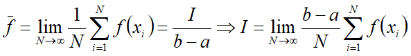
五、学习配位数Z计算

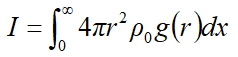
和对分布函数一起被提及的还有配位数这个概念，所谓的配位数就是4πr2ρ0g(r)与Y轴包围的面积。

在被积函数4πr^2ρ0g(r)相当复杂时，就只能采取数值积分的求法。选择采用大数定理：在（a,b）区域内均匀随机抽样得到N个点x1、x2、x3、...、xN;求这些点上被积函数的值f(x1)、f(x2)、f(x3)......f(xN)、f(x1)、于是f(x)在[a,b]区域的平均值：

fRAD= fit(r,g, '**oothingspline');

rgRAD=linspace(r(m(1)),r(m(end)),1000)';

rho=N/(height*width*long);

intgtotal_cal=rho*4*pi*rgRAD.^2.*fRAD(rgRAD);

z=(max(rgRAD)-min(rgRAD)).*(sum(intgtotal_cal))./1000;

以上就是由为了求对分布函数图像而衍生出来的相关计算。

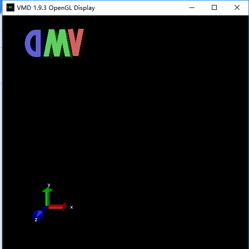
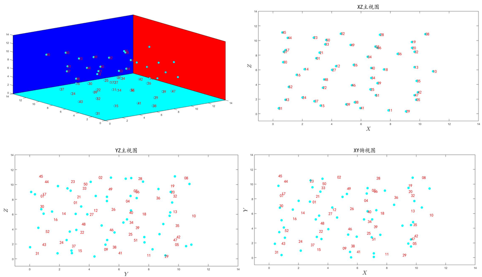
六、掌握时间演化轨迹图

我们得到的体系原子坐标数据是时间演化的轨迹图像，但是实际在过动力学模拟的时候我们并没有看见体系的演化轨迹。所以我们就应该尝试一下用matlab看演化轨迹图。该问题比较简单利用得到的原子坐标进行简单的处理，再和matlab动态绘图相结合就得到了轨迹图，

clear

tic

height=11.1087999344000004;width=11.1087999344000004;long=11.1087999344000004;

N=52;

load('data.mat')

for i=1:length(a)/N

b= a(1 (N*(i-1)):N*i,:);

Centers{i,1}=b;

end

gg = 1;

figure1 =figure('Position',[395 86 894 700],'Name','Mg原子三维空间运动轨迹','NumberTitle','off','Color','w','Menubar','figure','WindowState','maximized');

axes1 = axes('Parent',figure1);

view(axes1,[-37.5 30]);2

for k=1:length(Centers)

centers=Centers{k,1};

fill3([0 14 14 0],[0 0 14 14],[0 0 0 0],[0 1 1],'Parent',axes1);

hold(axes1,'on');

fill3([0 14 14 0],[14 14 14 14],[0 0 14 14],[0 0 1],'Parent',axes1);

fill3([14 14 14 14],[0 0 14 14],[0 14 14 0],[1 0 0],'Parent',axes1);

plot3(centers(:,1),centers(:,2),centers(:,3),'Parent',axes1,'MarkerFaceColor',[0 1 1],'MarkerEdgeColor',[0 0.447058826684952 0.74117648601532],'MarkerSize',8,'Marker','o','LineStyle','none');

hold(axes1,'off');

str1=['01';'02';'03';'04';'05';'06';'07';'08';'09';'10';'11';'12';'13';'14';'15';'16';'17';'18';'19';'20';'21';'22';'23';'24';'25';'26';'27';'28';'29';'30';'31';'32';'33';'34';'35';'36';'37';'38';'39';'40';'41';'42';'43';'44';'45';'46';'47';'48';'49';'50';'51';'52'];

text(axes1,centers(:,1),centers(:,2),centers(:,3),str1,'FontSize',14,'fontname','楷体','Color','red');

fmat(:,k)=getframe; %拷贝祯到矩阵fmat中

im = frame2im(getframe);

[I,map] = rgb2ind(im,256);

if gg == 1

imwrite(I,map,'lxx.gif','GIF', 'Loopcount',inf,'DelayTime',0.05);

gg = gg 1;

else

imwrite(I,map,'lxx.gif','WriteMode','append','DelayTime',0.05);

end

%% 主视图XZ

figure1 = figure('Name','Mg原子三维空间运动轨迹-XZ主视图','NumberTitle','off','Color','w','Menubar','figure','WindowState','maximized');

axes1 = axes('Parent',figure1);

%hold(axes1,'on');

for k=1:length(Centers)

centers=Centers{k,1};

plot(centers(:,1),centers(:,3),'Parent',axes1,'MarkerFaceColor',[0 1 1],'MarkerEdgeColor',[0 1 1],'MarkerSize',8,'Marker','o','LineStyle','none');

text(axes1,centers(:,1),centers(:,3),str1,'FontSize',14,'fontname','楷体','Color','red');

xlim(axes1,[-1 14]);

ylim(axes1,[-1 14]);

box(axes1,'on');

ylabel(axes1,'$Z$','FontSize',20,'Interpreter','latex');

xlabel(axes1,'$X$','FontSize',20,'Interpreter','latex');

title('XZ主视图','FontSize',20,'FontName','楷体');

fmat(:,k)=getframe; %拷贝祯到矩阵fmat中

% im = frame2im(getframe);

% [I,map] = rgb2ind(im,256);

% if gg == 1

% imwrite(I,map,'lxx.gif','GIF', 'Loopcount',inf,'DelayTime',0.05);

% gg = gg 1;

% else

% imwrite(I,map,'lxx.gif','WriteMode','append','DelayTime',0.05);

% end

end

% 左视图YZ

figure1 = figure('Name','Mg原子三维空间运动轨迹-YZ主视图','NumberTitle','off','Color','w','Menubar','figure','WindowState','maximized');

axes1 = axes('Parent',figure1);

%hold(axes1,'on');

for k=1:length(Centers)

centers=Centers{k,1};

plot(centers(:,2),centers(:,3),'Parent',axes1,'MarkerFaceColor',[0 1 1],'MarkerEdgeColor',[0 1 1],'MarkerSize',8,'Marker','o','LineStyle','none');

text(axes1,centers(:,1),centers(:,3),str1,'FontSize',14,'fontname','楷体','Color','red');

xlim(axes1,[-1 14]);

ylim(axes1,[-1 14]);

box(axes1,'on');

ylabel(axes1,'$Z$','FontSize',20,'Interpreter','latex');

xlabel(axes1,'$Y$','FontSize',20,'Interpreter','latex');

title('YZ左视图','FontSize',20,'FontName','楷体');

fmat(:,k)=getframe; %拷贝祯到矩阵fmat中

% im = frame2im(getframe);

% [I,map] = rgb2ind(im,256);

% if gg == 1

% imwrite(I,map,'lxx.gif','GIF', 'Loopcount',inf,'DelayTime',0.05);

% gg = gg 1;

% else

% imwrite(I,map,'lxx.gif','WriteMode','append','DelayTime',0.05);

% end

end

% 俯视图 XY

figure1 = figure('Name','Mg原子三维空间运动轨迹-YZ主视图','NumberTitle','off','Color','w','Menubar','figure','WindowState','maximized');

axes1 = axes('Parent',figure1);

%hold(axes1,'on');

for k=1:length(Centers)

centers=Centers{k,1};

plot(centers(:,1),centers(:,2),'Parent',axes1,'MarkerFaceColor',[0 1 1],'MarkerEdgeColor',[0 1 1],'MarkerSize',8,'Marker','o','LineStyle','none');

text(axes1,centers(:,1),centers(:,2),str1,'FontSize',14,'fontname','楷体','Color','red');

xlim(axes1,[-1 14]);

ylim(axes1,[-1 14]);

box(axes1,'on');

ylabel(axes1,'$Y$','FontSize',20,'Interpreter','latex');

xlabel(axes1,'$X$','FontSize',20,'Interpreter','latex');

title('XY俯视图','FontSize',20,'FontName','楷体');

fmat(:,k)=getframe; %拷贝祯到矩阵fmat中

% im = frame2im(getframe);

% [I,map] = rgb2ind(im,256);

% if gg == 1

% imwrite(I,map,'lxx.gif','GIF', 'Loopcount',inf,'DelayTime',0.05);

% gg = gg 1;

% else

% imwrite(I,map,'lxx.gif','WriteMode','append','DelayTime',0.05);

% end

end

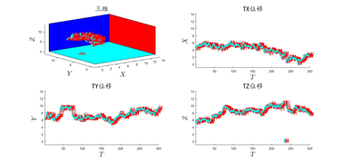
多个原子的运动轨迹看起来特别的乱，我们也可以追踪某一个原子的的运动轨迹绘制这样的图像。红色是标号01，绿色代表的是坐标

%原子运动轨迹追踪图

figure1 = figure('Name','Mg原子三维空间运动轨迹-YZ主视图','NumberTitle','off','Color','w','Menubar','figure','WindowState','maximized');

subplot1 = subplot(2,2,1,'Parent',figure1);

view(subplot1,[-37.5 30]);

subplot2 = subplot(2,2,2,'Parent',figure1);

subplot3 = subplot(2,2,3,'Parent',figure1);

subplot4 = subplot(2,2,4,'Parent',figure1);

hold(subplot1,'on');

hold(subplot2,'on');

hold(subplot3,'on');

hold(subplot4,'on');

fill3([0 14 14 0],[0 0 14 14],[0 0 0 0],[0 1 1],'Parent',subplot1);

fill3([0 14 14 0],[14 14 14 14],[0 0 14 14],[0 0 1],'Parent',subplot1);

fill3([14 14 14 14],[0 0 14 14],[0 14 14 0],[1 0 0],'Parent',subplot1);

xlim(subplot1,[-1 14]);

ylim(subplot1,[-1 14]);

zlim(subplot1,[-1 14]);

ylabel(subplot1,'$Y$','FontSize',20,'Interpreter','latex');

xlabel(subplot1,'$X$','FontSize',20,'Interpreter','latex');

zlabel(subplot1,'$Z$','FontSize',20,'Interpreter','latex');

title(subplot1,'三维','FontSize',20,'FontName','楷体');

xlim(subplot2,[1 length(Centers)]);

ylim(subplot2,[-1 14]);

ylabel(subplot2,'$X$','FontSize',20,'Interpreter','latex');

xlabel(subplot2,'$T$','FontSize',20,'Interpreter','latex');

title(subplot2,'TX位移','FontSize',20,'FontName','楷体');

xlim(subplot3,[1 length(Centers)]);

ylim(subplot3,[-1 14]);

ylabel(subplot3,'$Y$','FontSize',20,'Interpreter','latex');

xlabel(subplot3,'$T$','FontSize',20,'Interpreter','latex');

title(subplot3,'TY位移','FontSize',20,'FontName','楷体');

xlim(subplot4,[1 length(Centers)]);

ylim(subplot4,[-1 14]);

ylabel(subplot4,'$Z$','FontSize',20,'Interpreter','latex');

xlabel(subplot4,'$T$','FontSize',20,'Interpreter','latex');

title(subplot4,'TZ位移','FontSize',20,'FontName','楷体');

for k=1:length(Centers)

centers=Centers{k,1};

plot3(centers(1,1),centers(1,2),centers(1,3),'Parent',subplot1,'MarkerFaceColor',[0 1 1],'MarkerEdgeColor',[0 1 1],'MarkerSize',4,'Marker','o','LineStyle','none');

str1=['01'];

text(subplot1,centers(1,1),centers(1,2),centers(1,3),str1,'FontSize',14,'fontname','楷体','Color','red');

plot(k,centers(1,1),'Parent',subplot2,'MarkerFaceColor',[0 1 1],'MarkerEdgeColor',[0 1 1],'MarkerSize',4,'Marker','o','LineStyle','none');

str1=['01'];

text(subplot2,k,centers(1,1),str1,'FontSize',14,'fontname','楷体','Color','red');

plot(k,centers(1,2),'Parent',subplot3,'MarkerFaceColor',[0 1 1],'MarkerEdgeColor',[0 1 1],'MarkerSize',4,'Marker','o','LineStyle','none');

str1=['01'];

text(subplot3,k,centers(1,2),str1,'FontSize',14,'fontname','楷体','Color','red');

plot(k,centers(1,3),'Parent',subplot4,'MarkerFaceColor',[0 1 1],'MarkerEdgeColor',[0 1 1],'MarkerSize',4,'Marker','o','LineStyle','none');

str1=['01'];

text(subplot4,k,centers(1,3),str1,'FontSize',14,'fontname','楷体','Color','red');

fmat(:,k)=getframe; %拷贝祯到矩阵fmat中